4.3 Distributed Lag Models
Consider a response time series \(y_t\) and an input (or “exposure”) time series \(x_t\). There may be other covariates of interest that merit consideration be we will ignore them for now and discuss their inclusion in the next section. We will consider models of the form
\[ y_t = \sum_{j=-\infty}^\infty \beta_j x_{t-j} + \varepsilon_t \] where \(\varepsilon\) represents an iid noise process. In continuous time settings, this model might be written as
\[ y(t) = \int_{-\infty}^\infty \beta(u)x(t-u)\,du + \varepsilon(t) \] and the function \(h(u)\) is called the impulse-response function. We will focus on the discrete version of the model here as we will be working with discrete data. In that case the collection \(\{\beta_j\}\) as a function of the lag \(j\) will be referred to as the distributed lag function.
There is a special class of problems that we will consider that makes two assumptions. The first is that \(\beta_j=0\) if \(j < 0\). This assumption produces what is called a physically realizable or causal system because it does not depend on knowing future values of \(x_t\). Another key property that we may assume about the collection \(\{\beta_j\}\) is that
\[ \sum_{j=0}^\infty |\beta_j| < \infty \]
which is sufficient for producing a linear system that is stable. In other words, a bounded input \(x_t\) will produce a bounded output \(y_t\).
As written above, each \(y_t\) is a function of the infinite past. In practice we will assume that for some \(M>0\), \(\beta_j=0\) for all \(j > M\).
To see how this model works, let’s consider a hypothetical time series
\[\begin{eqnarray*} & \vdots &\\ x_{t-3} & = & 0\\ x_{t-2} & = & 0\\ x_{t-1} & = & 0\\ x_t & = & 1\\ x_{t+1} & = & 0\\ x_{t+2} & = & 0\\ x_{t+3} & = & 0\\ & \vdots & \end{eqnarray*}\]
so at time \(t\) there is a single unit spike and the series is equal to 0 at all other time. This can be thought of as an input “shock”. Then the model implies that
\[\begin{eqnarray*} \mathbb{E}[y_t] & = & \sum_{j=0}^\infty \beta_jx_{t-j}\\ & = & \beta_0x_t + \beta_1\times 0 + \beta_2\times 0 + \cdots\\ & = & \beta_0\\ \mathbb{E}[y_{t+1}] & = & \beta_0\times 0 + \beta_1x_t + \beta_2\times 0 + \beta_3\times 0 + \cdots\\ & = & \beta_1\\ \mathbb{E}[y_{t+2}] & = & \beta_0\times 0 + \beta_1\times 0 + \beta_2x_t + \beta_3\times 0 + \cdots\\ & = & \beta_2\\ & \vdots & \\ \mathbb{E}[y_{t+M}] & = & \beta_M \end{eqnarray*}\]
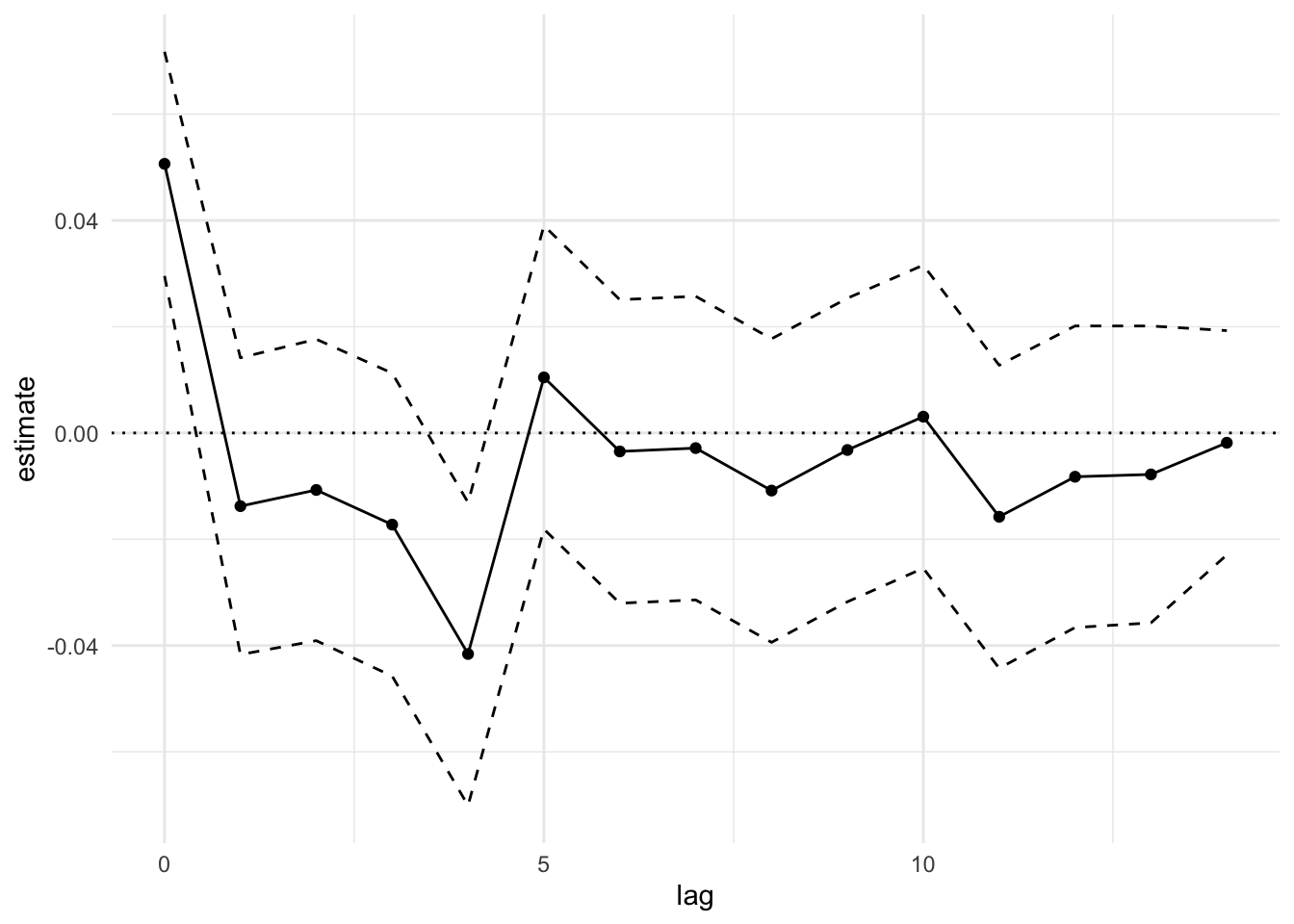
Therefore, the sequence \(\beta_0, \beta_1, \beta_2,\dots\) represents the expected values of the outcome sequence at time \(t, t+1, t+2, \dots\). A useful plot is a plot of the \(\beta_j\) vs. \(j\) to see how the effect of a unit spike in \(x_t\) is distributed over time.
Given a distributed lag model, a sometimes useful summary statistic is \[ \eta = \sum_{j=0}^M \beta_j. \] The value \(\eta\) is sometimes interpretable as a “cumulative effect”, particularly when the outcome is a count outcome. If we have \(\beta_j\ne 0\) and \(\eta\approx 0\), then that might suggest that on average across \(M\) time points, the effect of a unit increase in \(x_t\) is roughly zero. For example, in the “mortality displacement” hypothesis described above, one might hypothesize that \(\eta=0\), so that the cumulative number of excess deaths is \(0\) over \(M\) time points. Whether this is a useful interpretation or not will depend on the context in which the analysis is done.
4.3.1 Example: Baltimore Temperature and Mortality
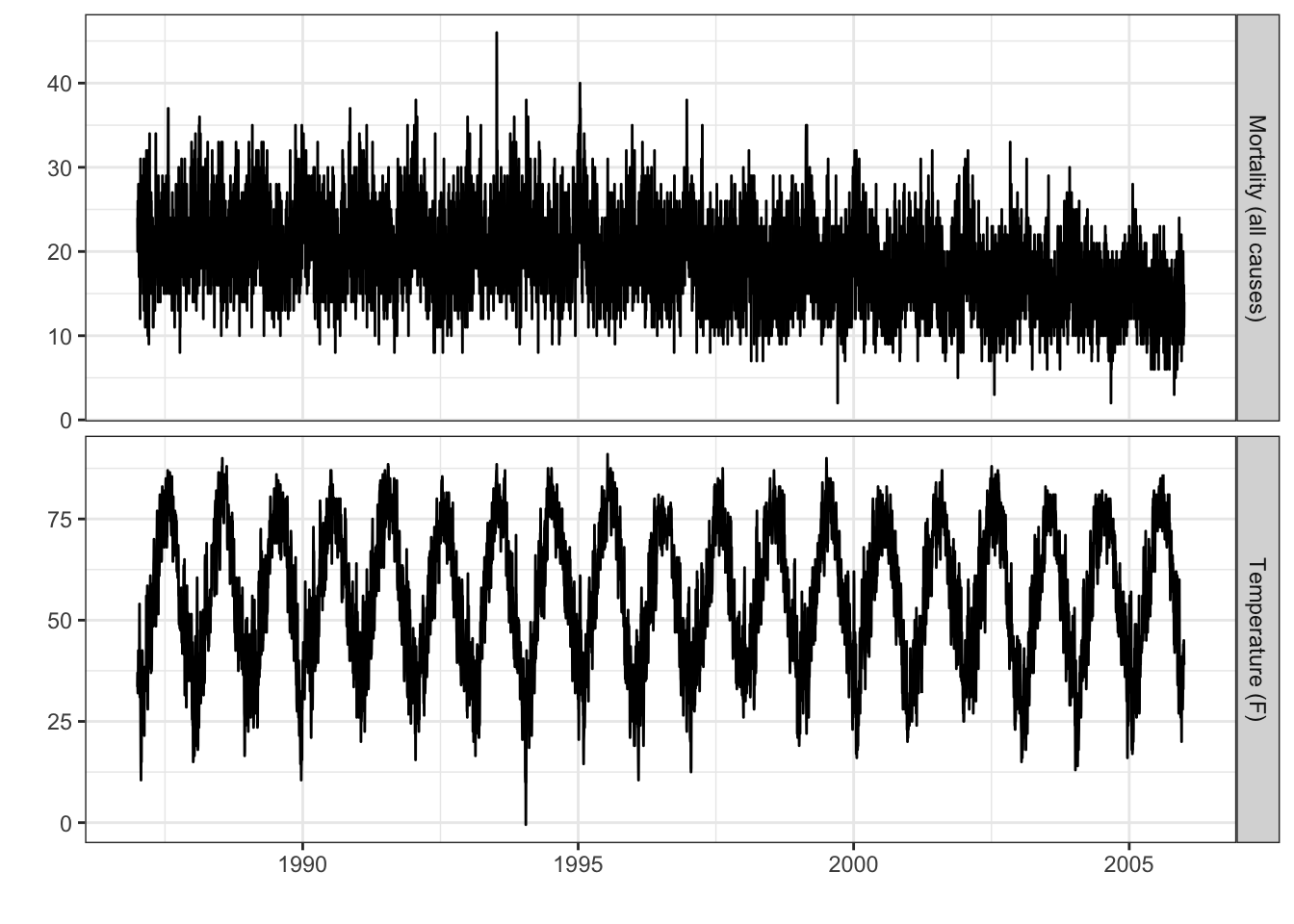
The following plot shows daiy temperature and mortality data for Baltimore, MD (USA) for the years 1987–2005.
Below is a scatter plot of daily temperature and mortality for the same time period in Baltimore.
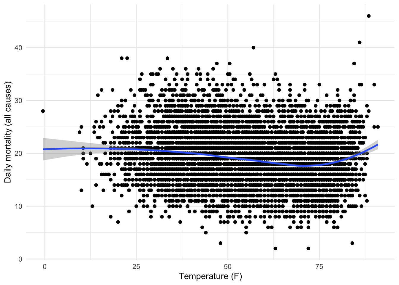
A few interesting things pop out here:
In general, higher temperatures are correlated with lower mortality.
Except, if the temperature gets too high, then they are correlated with higher mortality
There is a suggestion here that we may need to separate out different time scales of variation to look at the temperature-mortality relationship.
# A tibble: 3 x 5
  term          estimate std.error statistic  p.value
  <chr>            <dbl>     <dbl>     <dbl>    <dbl>
1 (Intercept)      24.1      0.507      47.5 0.
2 ns(tempF, 2)1   -10.3      0.987     -10.4 4.16e-25
3 ns(tempF, 2)2    -3.19     0.251     -12.7 1.10e-36
# A tibble: 16 x 5
term estimate std.error statistic p.value
<chr> <dbl> <dbl> <dbl> <dbl>
1 (Intercept) 23.1 0.222 104. 0
2 Lag(tempF, 0:14)0 0.0506 0.0108 4.71 0.00000258
3 Lag(tempF, 0:14)1 -0.0138 0.0142 -0.967 0.334
4 Lag(tempF, 0:14)2 -0.0107 0.0145 -0.741 0.459
5 Lag(tempF, 0:14)3 -0.0172 0.0145 -1.19 0.236
6 Lag(tempF, 0:14)4 -0.0416 0.0145 -2.86 0.00426
7 Lag(tempF, 0:14)5 0.0105 0.0146 0.718 0.473
8 Lag(tempF, 0:14)6 -0.00348 0.0146 -0.239 0.811
9 Lag(tempF, 0:14)7 -0.00285 0.0146 -0.195 0.845
10 Lag(tempF, 0:14)8 -0.0108 0.0146 -0.744 0.457
11 Lag(tempF, 0:14)9 -0.00320 0.0146 -0.220 0.826
12 Lag(tempF, 0:14)10 0.00307 0.0146 0.211 0.833
13 Lag(tempF, 0:14)11 -0.0158 0.0145 -1.08 0.278
14 Lag(tempF, 0:14)12 -0.00824 0.0145 -0.569 0.569
15 Lag(tempF, 0:14)13 -0.00780 0.0143 -0.548 0.584
16 Lag(tempF, 0:14)14 -0.00184 0.0108 -0.171 0.864