2.8 Autocorrelation

One summary statistic of a stationary time series is the auto-correlation function, or the ACF. This is simply the auto-covariance function \(\gamma(k)\) divided by \(\gamma(0)\). As a result, the ACF(0) is always 1 and usually we plot that even thought it’s the same every time.

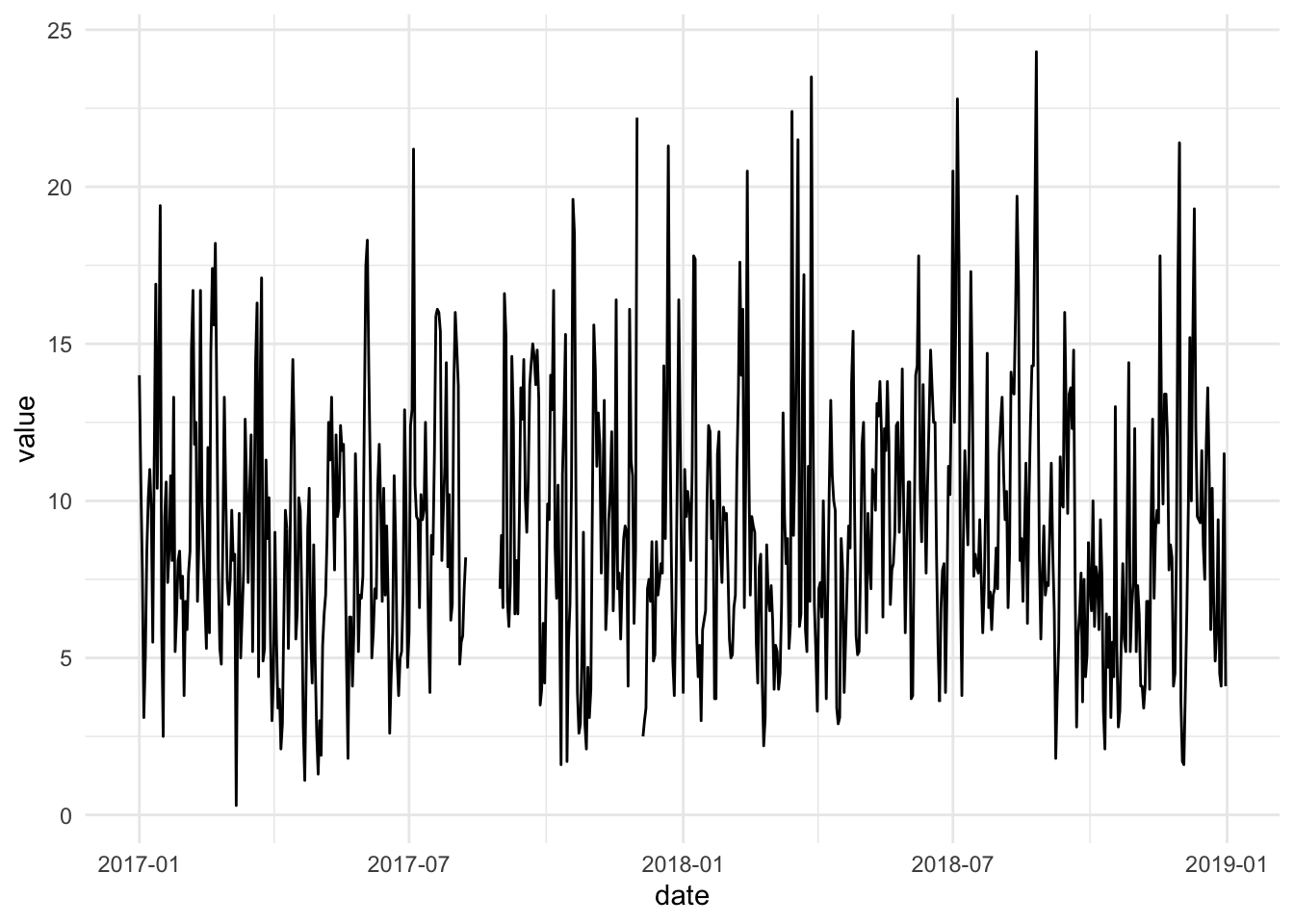
Here is the raw St. Louis particulate matter data for 2017–2018.

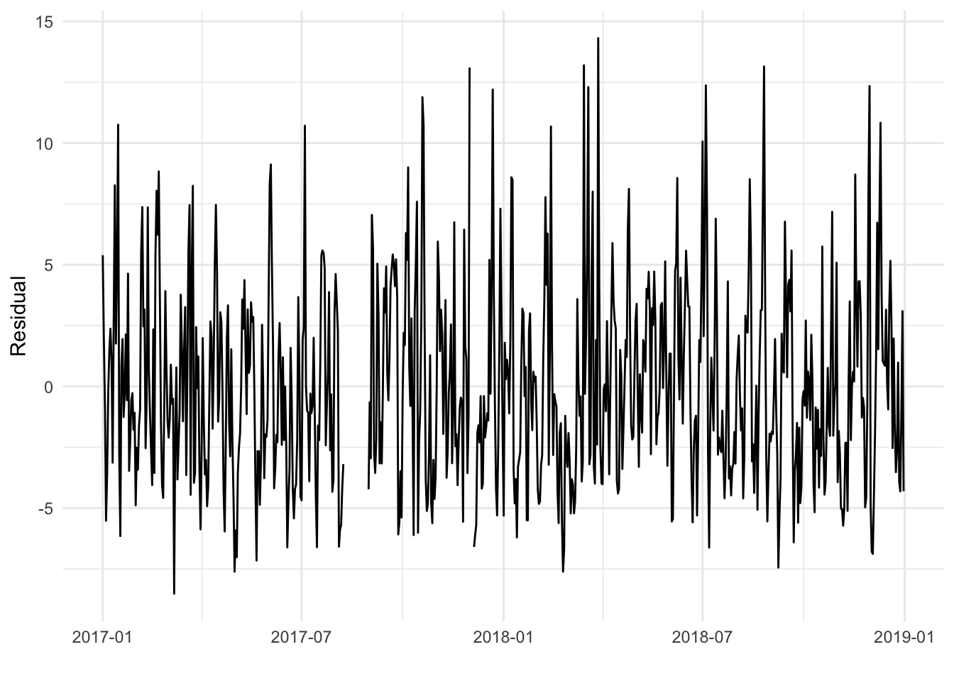
Let’s remove a smooth and monthly average cyclic trend from the data and look at the residuals.

Here’s the auto-correlation function for the St. Louis data, after removing the trend and monthly effects.

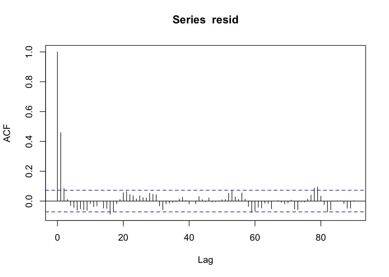
We can see that there appears to be some correlation leftover at lags of 1 day but the correlations at the remaining lags are close to zero.

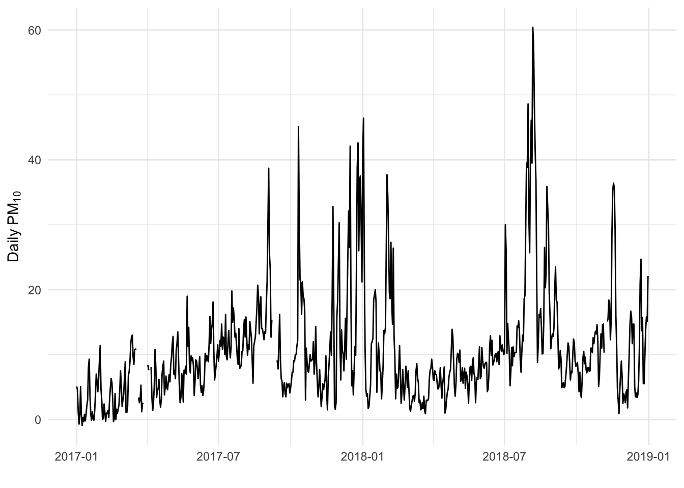
In contrast to the St. Louis data, here is the Fresno data.

What you don’t want to see is something like below. This is the ACF on the raw Fresno data.

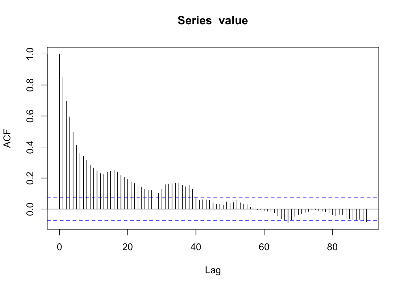
The question here then is why is there such strong autocorrelation at lags 1, 2, 3, …? The problem is that the data cannot answer that question. It could either be a truly random autocorrelation in the series or there is a fixed effect or trend that hasn’t been removed (i.e. the series is not stationary).

This pattern in the ACF plot is usually an indication of non-stationarity rather than a sign of interesting auto-correlation. If you see something like this, you should check to see if your time series demonstrates any strong fixed effects, like a linear trend or a seasonal component. If they do, those effects should be removed first (e.g. via regression modeling) and the ACF plot re-plotted.

As another example, here is the ACF plot of the residuals from the Baltimore temperature data shown in the last section, after removing a monthly mean.

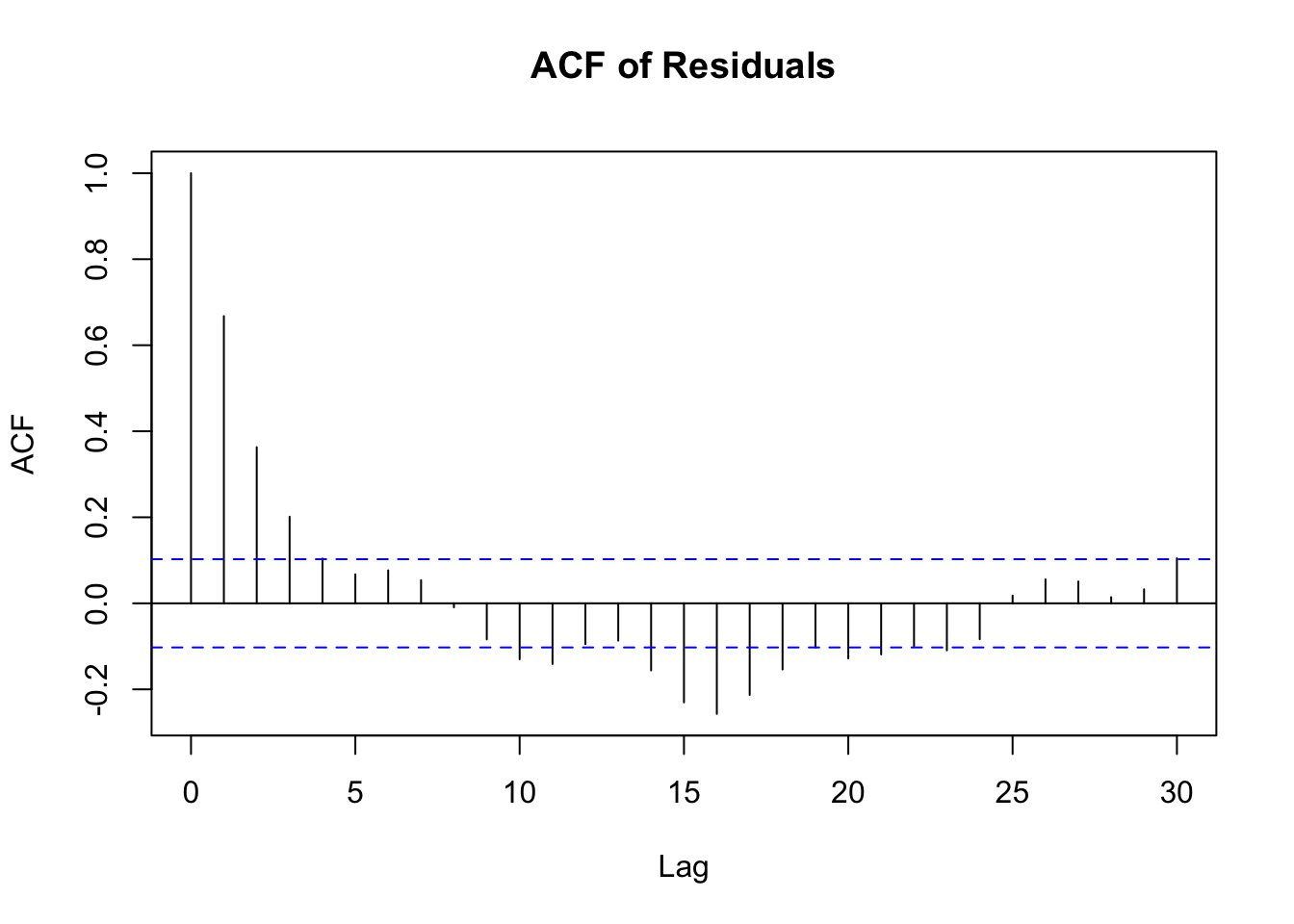
The ACF plot clearly shows there is some short-term auto-correlation left in the residuals. What to do about this will depend on the application and question at hand and we will discuss this further in the section on time series regression modeling.