5.7 Example: Tracking the Position of a Car

The model we will employ here will be an extension of the model for the spacecraft mentioned previously. The goal is to track the linear (one-dimensional) position of a car traveling down a straight road. The position of the car along this road at time \(t\) is \(p_t\) and is modeled as

\[ p_t = p_{t-1} + v_{t-1}\Delta t + \frac{1}{2}a_{t-1} \Delta t^2 + w_t \]

where \(v_{t-1}\) is the velocity, \(a_{t-1}\) is the acceleration, \(\Delta t\) is the time difference between measured time points, and \(w_t\) is a noise term. In this case we can write the state vector as

\[ x_t = [p_t, v_t, a_t]. \]

If we let

\[ \Theta = \left[\begin{array}{ccc} 1 & \Delta t & \frac{1}{2}\Delta t^2\\ 0 & 1 & \Delta t\\ 0 & 0 & \alpha \end{array} \right] \] where \(\alpha\) is a (known) coefficient characterizing the state transition for the acceleration term, then the state equation is

\[ x_t = \Theta x_{t-1} + w_t \] where \(w_t\sim\mathcal{N}(0, \tau^2I)\).

For the data, we have two observations. One is a GPS coordinate (the longitude in this case) indicating the position in one dimension and the other is the acceleration in the direction of the car. Acceleration can be in the forward direction (positive) or the backwards direction (negative). The data are the represented as

\[ y_t = Ax_t + v_t \]

where

\[ A = \left[\begin{array}{ccc} 1 & 0 & 0\\ 0 & 0 & 1 \end{array} \right] \] There are no direct measurements of velocity.

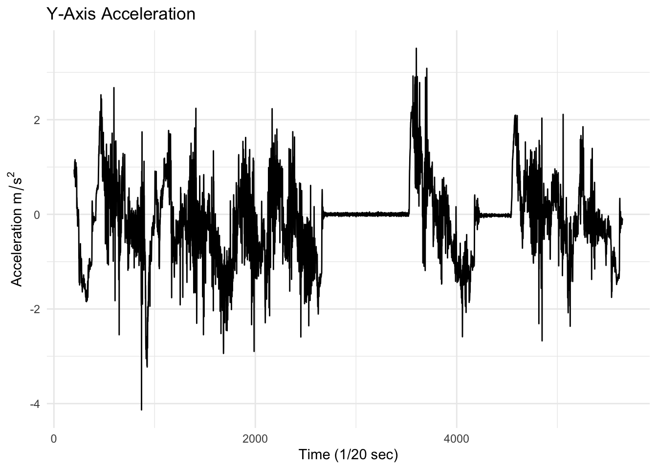
Here is the y-axis acceleration (in \(m/s^2\)) of the car over time. The y-axis in this case is the direction of travel.

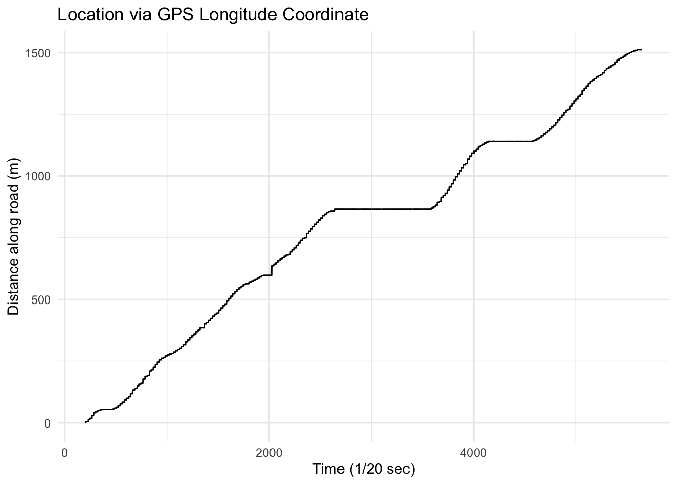
Here is the longitude position of the car over time, converted into a distance in meters along the road. The sampling rate of the data was 20 Hz (20 measurements per second) so the x-axis of the plot is in 1/20ths of a second.

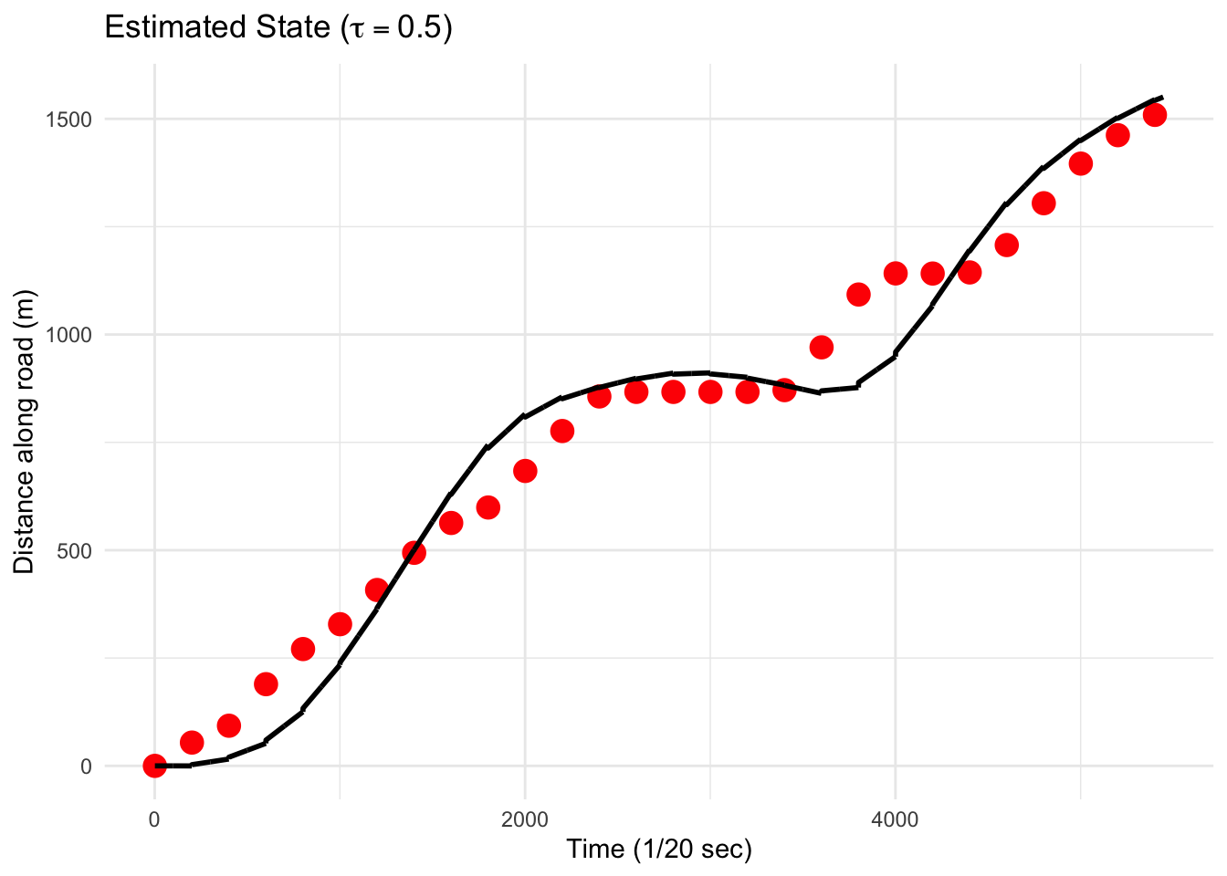
The actual observed GPS measurements are taken at 20 Hz, but we may confront situations where the data cannot be measured so frequently. For example, the acceleration is an inertial measurement that is always available, but the GPS measurements rely on satellites that may or may not be available at all times. In order to simulate possible lack of data, we can downsample the GPS data by downsampling the data. Here, we only keep one of every 1,000 GPS values. The results of the Kalman filtering algorithm are shown below.

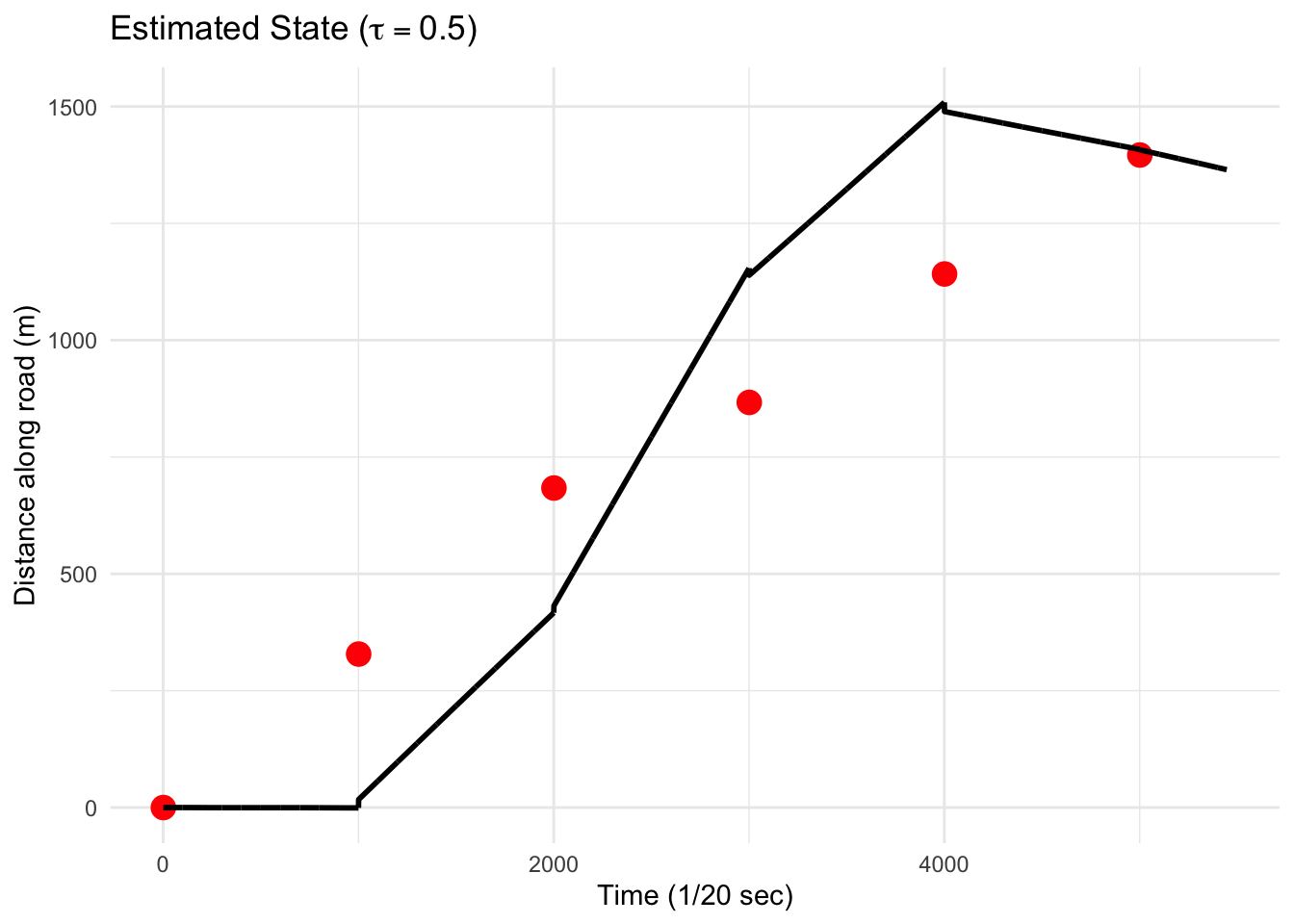
In the plot above we set \(\tau = 0.5\) and \(\sigma=20\). Also, \(\alpha\) was set to \(0.64\).

Below is a plot where we downsample less and keep one of every 200 GPS values.

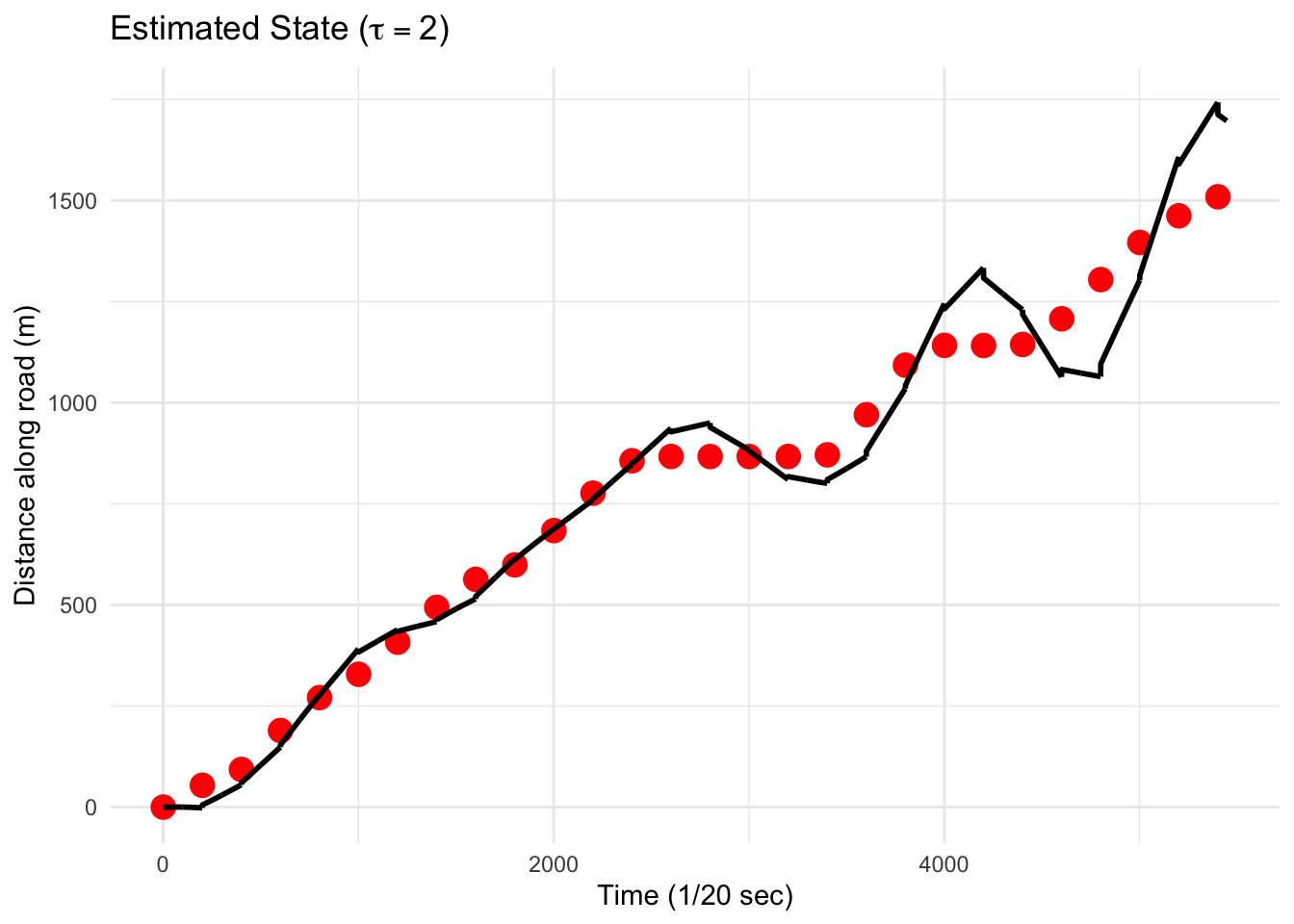
We can see that the estimate state tries to keep up with the GPS values when they are available but generally takes time to correct itself. In the above plot we had \(\tau=2\) but we can alter the correction behavior by decreasing \(\tau\). In the next plot we have \(\tau=0.5\) and we can see the track is much smoother.

Although the estimate state is smoother, it is also more biased. Therefore, when choosing the tuning parameters \(\tau\) and \(\sigma\), one needs to balance the need for accuracy and the need for smoothness (bias vs. variance).