3.4 Spectral Analysis
The above derivation of Parseval’s theorem suggest that there may be some value to examining the values of \(R_p^2/2\) as a function of \(p\). Roughly speaking (modulo a few constants of proportionality), a plot of \(R_p^2/2\) vs. \(p\) is called the raw periodogram and is a plot of the energy in each frequency range as a function of the frequency. If we let \(\omega_p=2\pi p/n\), then the periodogram is \[ I(\omega_p) = \frac{n}{4\pi} R^2_p. \]
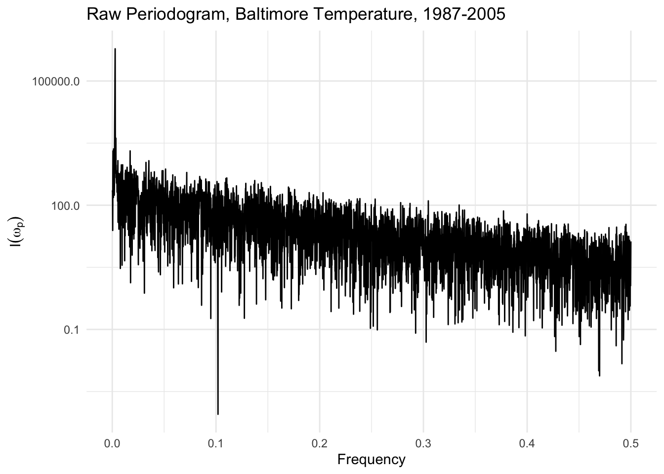
Before going too much further, it’s worth noting that we haven’t really done anything to reduce the complexity of the data, i.e. we haven’t modeled anything. Plotting the periodogram as a function of \(\omega_p\) shows a very noisy function. Furthermore, the estimate of \(I(\omega_p)\) does not get less noisy as we increase the sample size \(n\). Intuitively, this is because the “model” that we started out with here had \(n\) parameters for \(n\) data points. Therefore, as we increase \(n\), we simply increase the number of parameters that we need to estimate. This problem can be solved via smoothing, which we will discuss later.
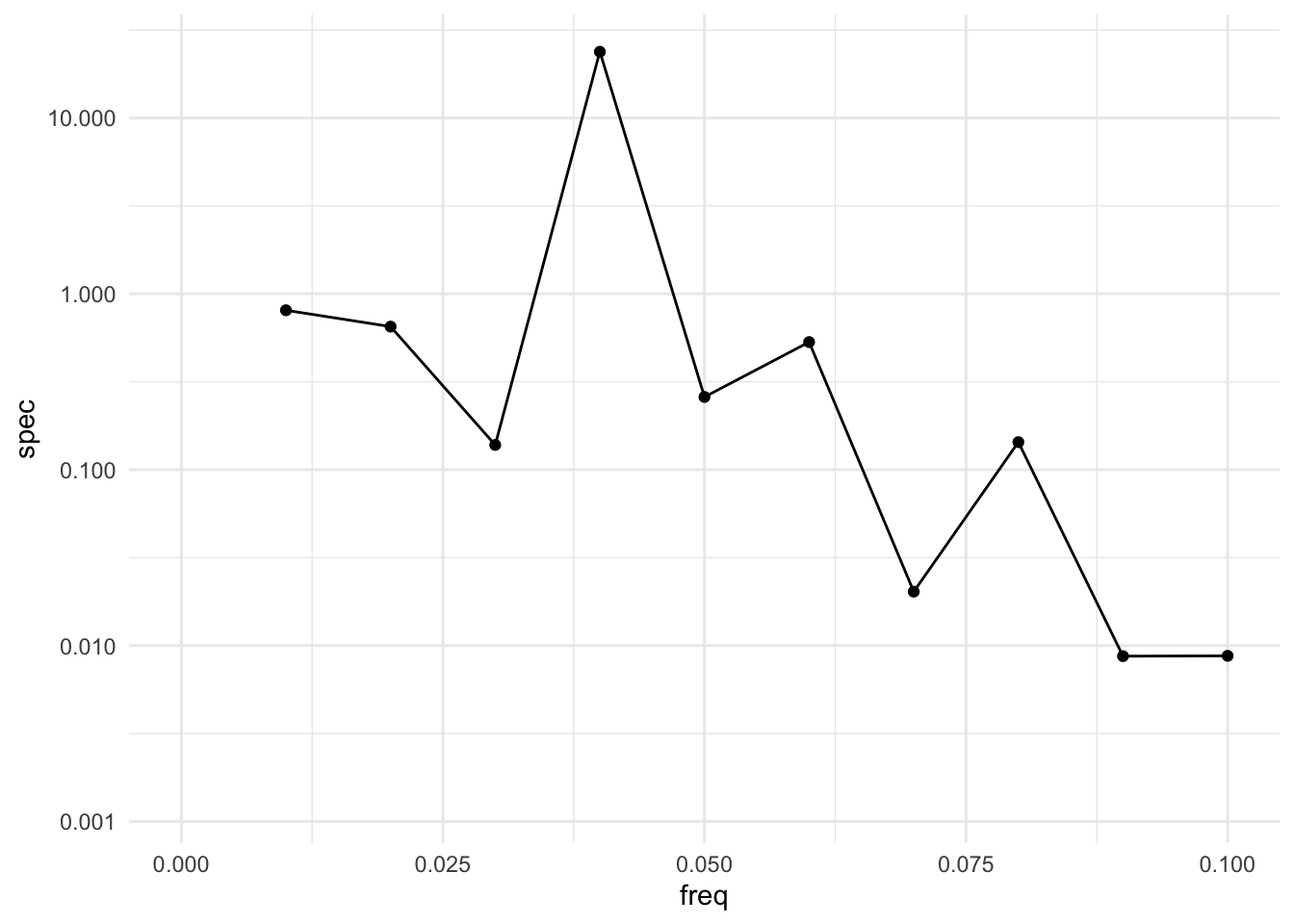
The raw periodogram can be obtained via the spectrum() function in R, which computes the periodogram using the Fast Fourier Transform (see below). We can plot the raw periodogram for the Baltimore temperature data below.
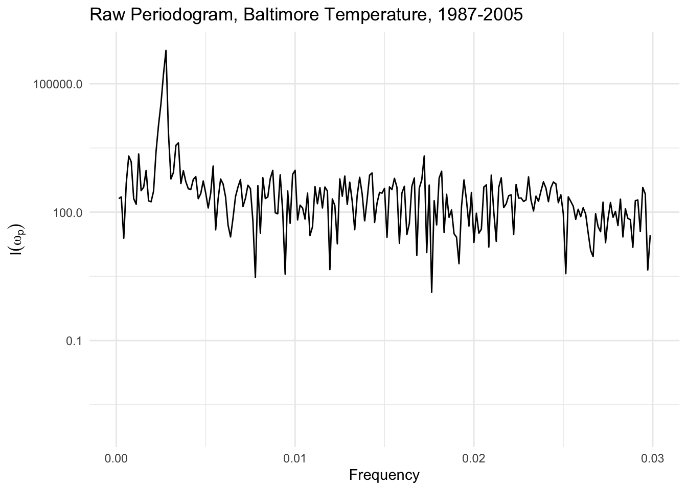
If we look more carefully at the spectrum, there is a large spike at frequency \(0.00278\), which comes out to a cycle with a period of \(1/0.00278 \approx 360\) days. Hence, we have re-discovered the annual cycle in the temperature data that we found previously with the linear model with the cosine terms.
Note also that the y-axis is presented on a log scale, which is conventional for a plot of the raw periodogram.
3.4.1 Smoothing the Periodogram
One problem with the raw periodogram is that it is not a consistent estimator of the the energy associated with a given frequency. In other words, the variability of the estimate of \(I(\omega_p)\) does not go to zero as the length of the time series \(n\rightarrow\infty\). Intuitively, this is clear because as \(n\rightarrow\infty\), we may have more data points but we also have more frequency coeffiients to estimate! So the number of parameters also increases with \(n\). Therefore, the plot of \(I(\omega_p)\) will get denser as \(n\rightarrow\infty\) becase there are more frequencies \(\omega_p\), but it will not become less noisy.
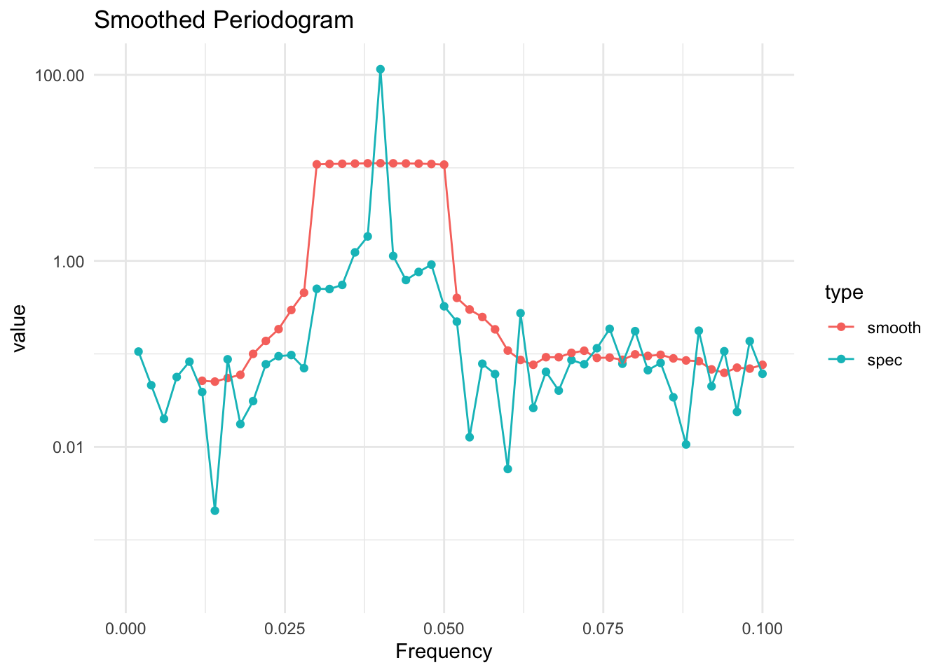
However, it turns out there is a simple way to produce a consistent estimate of \(I(\omega_p)\), and that is to smooth the estimate by averaging values of \(\hat{I}(\omega_p)\) with values at neighboring frequencies. This simple averaging is sufficient to produce an estimate whose variability goes to zero as \(n\rightarrow\infty\).
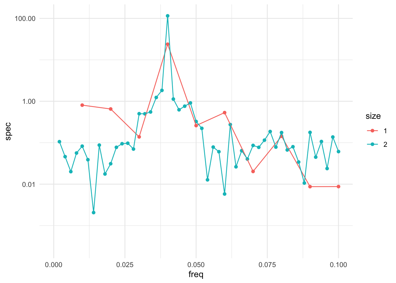
The only real issue with smoothing the periodogram is that you need to balance two goals
The size of the window that includes the neighboring values should increase with the sample size, to include more and more neighboring values.
The number of points in the window, relative to the total sample size, should go to zero.
In other words, the number of points in the window should increase, but not too fast. If the window contains \(m\) neighboring points, then using something like \(m\approx\sqrt{n}\) would work because \(m\rightarrow\infty\) as \(n\rightarrow\infty\) but \(m/n\rightarrow 0\) as \(n\rightarrow\infty\).