4.2 Filtering Time Series

In the model

\[ y_t=\sum_{j=-\infty}^\infty \beta_j x_{t-j} \]

the collection of \(\{\beta_j\}\) is called a linear filter. Clearly, \(y_t\) is a linear function of \(x_t\) and it is a filtered version of \(x_t\). Linear filtering, where \(\beta_j\) is a known collection of numbers, is often used to identify patterns and signals in a noisy time series (in this case \(x_t\)).

Filtering involves a convolution between two series \(x_t\) and \(\beta_j\). The convolved series is then called \(y_t\). At time \(t\), the convolution (in words) is the sum of the product between the the \(\beta_j\) series going forward and the \(x_t\) series going backwards.

\[ \begin{array}{ccccccccc} \cdots & x_{t+3}, & x_{t+2}, & x_{t+1}, & x_t, & x_{t-1}, & x_{t-2}, & x_{t-3} & \cdots\\ & \times & \times & \times & \times & \times & \times& \times & \\ \cdots & \beta_{-3}, & \beta_{-2}, &\beta_{-1}, & \beta_{0}, & \beta_{1}, & \beta_{2}, & \beta_{3} & \cdots\\ \end{array} \]

We will assume throughout that the \(\beta_j\)s satisfy the condition

\[ \sum_{j=-\infty}^\infty |\beta_j| < \infty \]

4.2.1 Fourier Transforms of Convolutions

Given the filtered time seres \(y_t\) specified as \[ y_t=\sum_{j=-\infty}^\infty \beta_j x_{t-j} \]

what is its Fourier transform?

\[\begin{eqnarray*} y_\omega & = & \sum_{t=-\infty}^\infty \sum_{j=-\infty}^\infty \beta_j x_{t-j}\exp(-2\pi i\omega t)\\ & = & \sum_{t=-\infty}^\infty \sum_{j=-\infty}^\infty \beta_j x_{t-j}\exp(-2\pi i\omega (t - j + j))\\ & = & \sum_{t=-\infty}^\infty \sum_{j=-\infty}^\infty \beta_j\exp(-2\pi i\omega\, j) x_{t-j}\exp(-2\pi i\omega (t - j))\\ & = & \sum_{j=-\infty}^\infty \beta_j\exp(-2\pi i\omega\, j) \sum_{t=-\infty}^\infty x_{t-j}\exp(-2\pi i\omega (t - j))\\ & = & \sum_{j=-\infty}^\infty \beta_j\exp(-2\pi i\omega\, j) \sum_{t=-\infty}^\infty x_{t}\exp(-2\pi i\omega \,t)\\ & = & \beta_\omega x_\omega \end{eqnarray*}\]

Here, the collection \(\beta_\omega\) as a function of \(\omega\) is called the transfer function and it is the Fourier transform of the impulse response function \(\beta_j\).

Why is this useful? For starters, this result provides an efficient way to compute the convolution between two series, which is exactly what is required with linear filtering. If we want to compute the filtered values \(y_1,y_2,\dots, y_n\), the naive formula requires us to compute the convolution formula \(n\) times, which has \(O(n^2)\) complexity. But instead, we can

1. Compute the Fourier transform \(x_\omega\) via the FFT for frequencies \(\omega = 0/n, 1/n, \dots, 1/2\).

2. Compute the FFT \(\beta_\omega\) for frequencies \(\omega = 0/n, 1/n, \dots, 1/2\).

3. Compute \(y_\omega = \beta_\omega x_\omega\) for frequencies \(\omega = 0/n, 1/n, \dots, 1/2\).

4. Compute the inverse FFT for all \(y_\omega\) to get the filtered values \(y_t\).

4.2.2 Low-Pass Filter

Consider the following simple (simulated) time series, which is a simple linear trend plus some Gaussian noise.

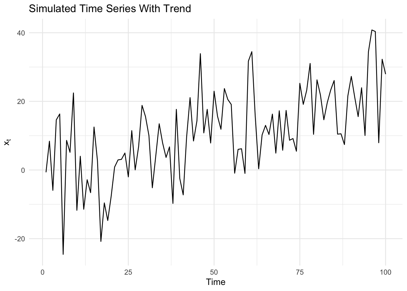
What will the output series look like if we convolve the original data with the following linear filter?

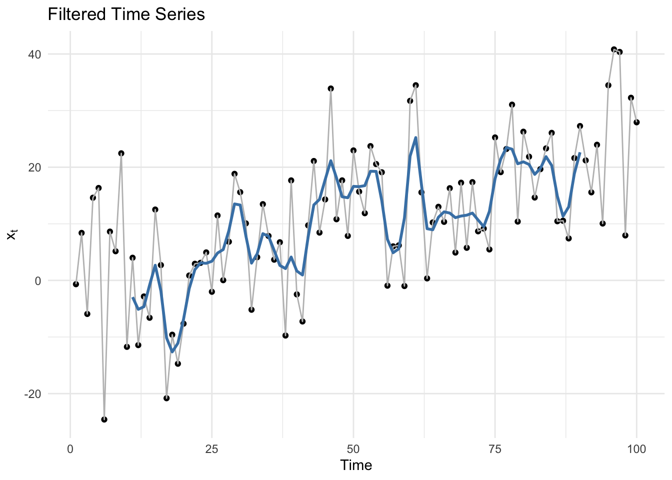
The answer is in the plot below in blue. The blue line shows the filtered series, which we can see is a smoother version of the original data. The filter shown above is a low-pass filter, which dampens higher frequencies in the data and allows lower frequencies to “pass” through.

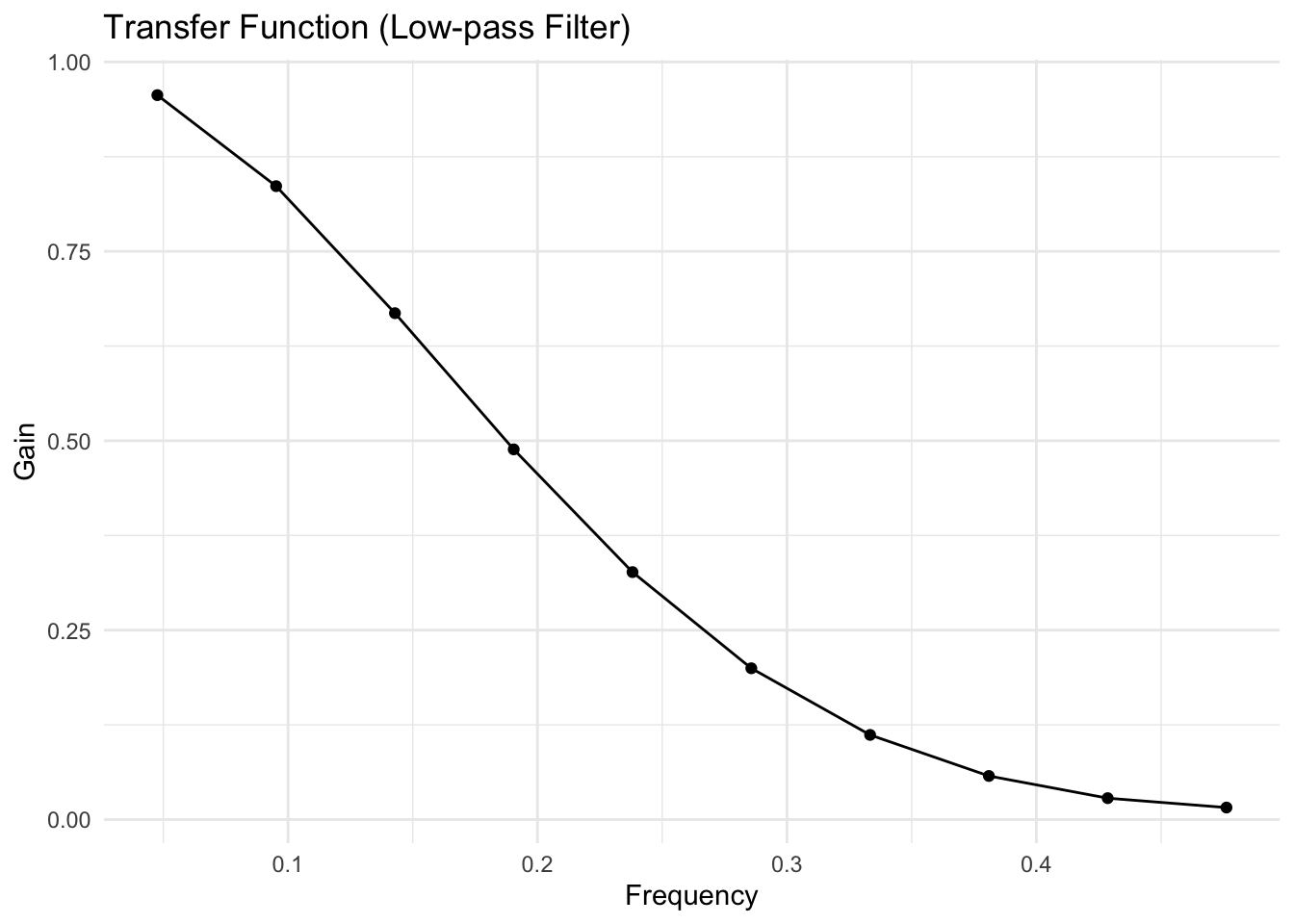
We can see the low-pass nature of the filter by examining the transfer function below. Here, we can see that the lower frequencies (near \(f=0\)) are given greater weight than the higher frequencies.

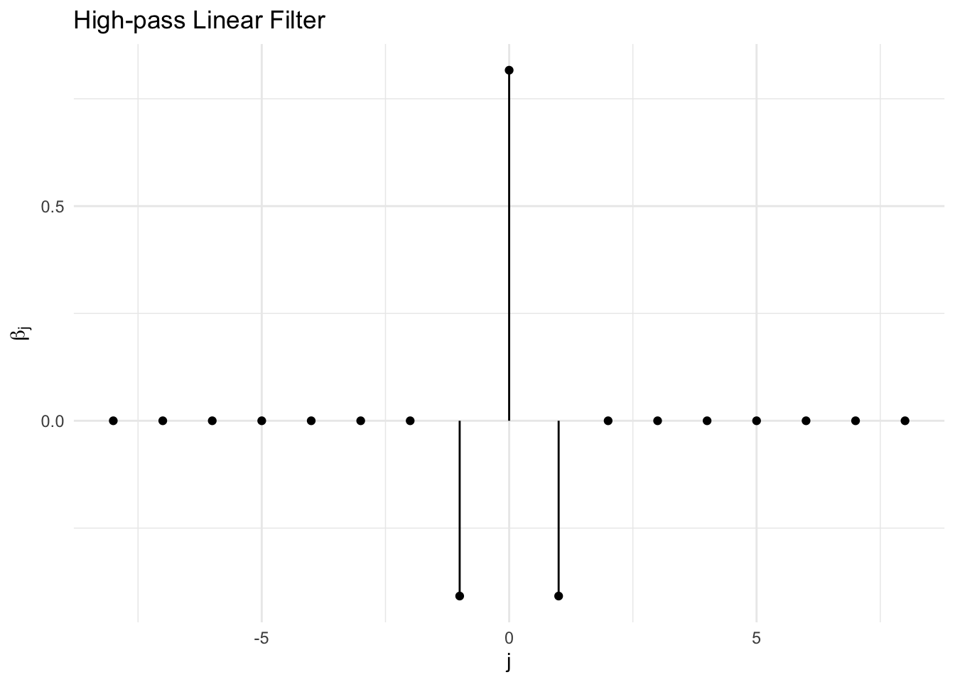
4.2.3 High-Pass Filter

The following is an example of a linear filter that dampens low frequencies and allows high frequencies to pass.

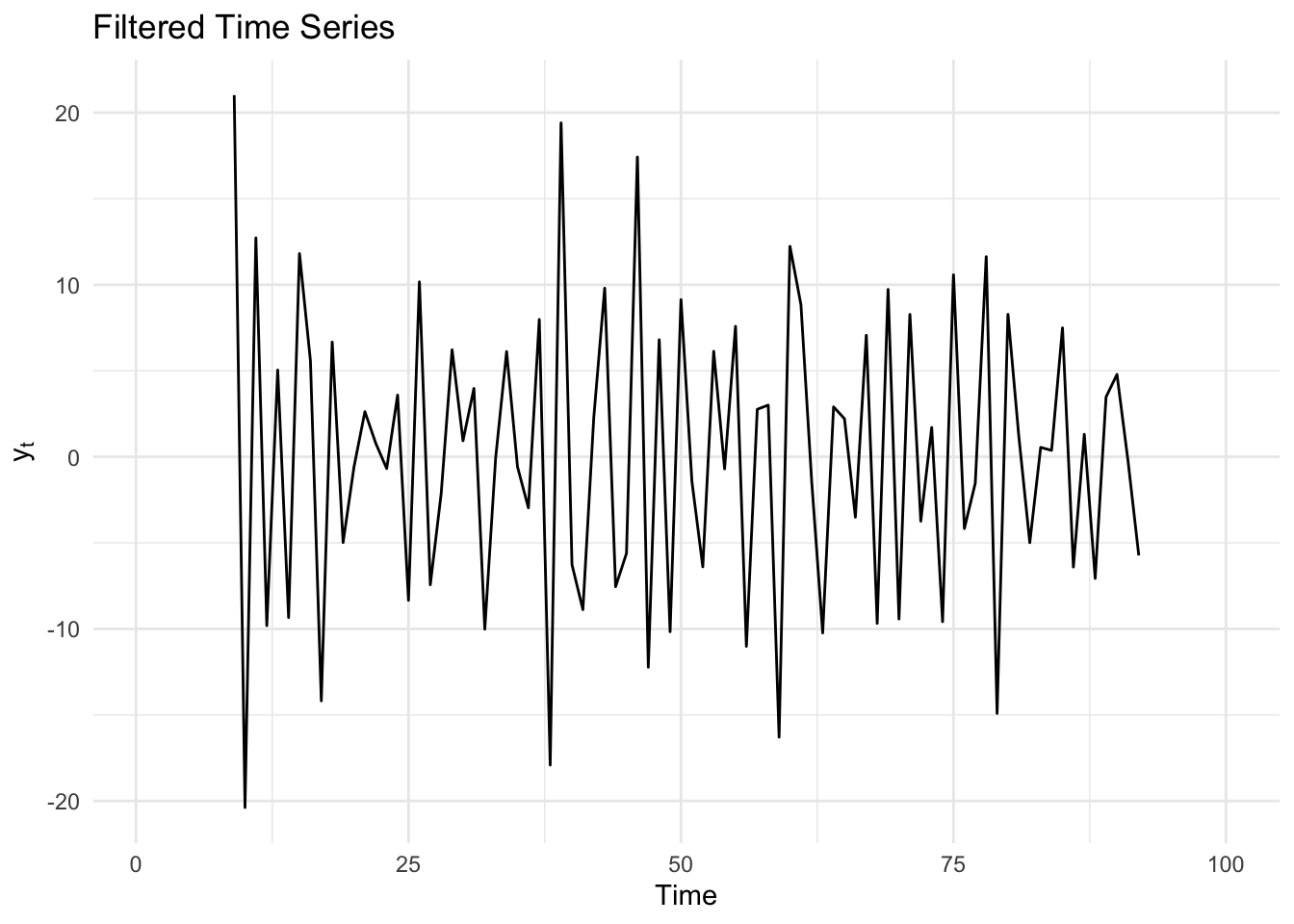
Here is the filtered version of the original data, using the high-pass filter. You can see that it looks like a series of residuals with the trend removed.

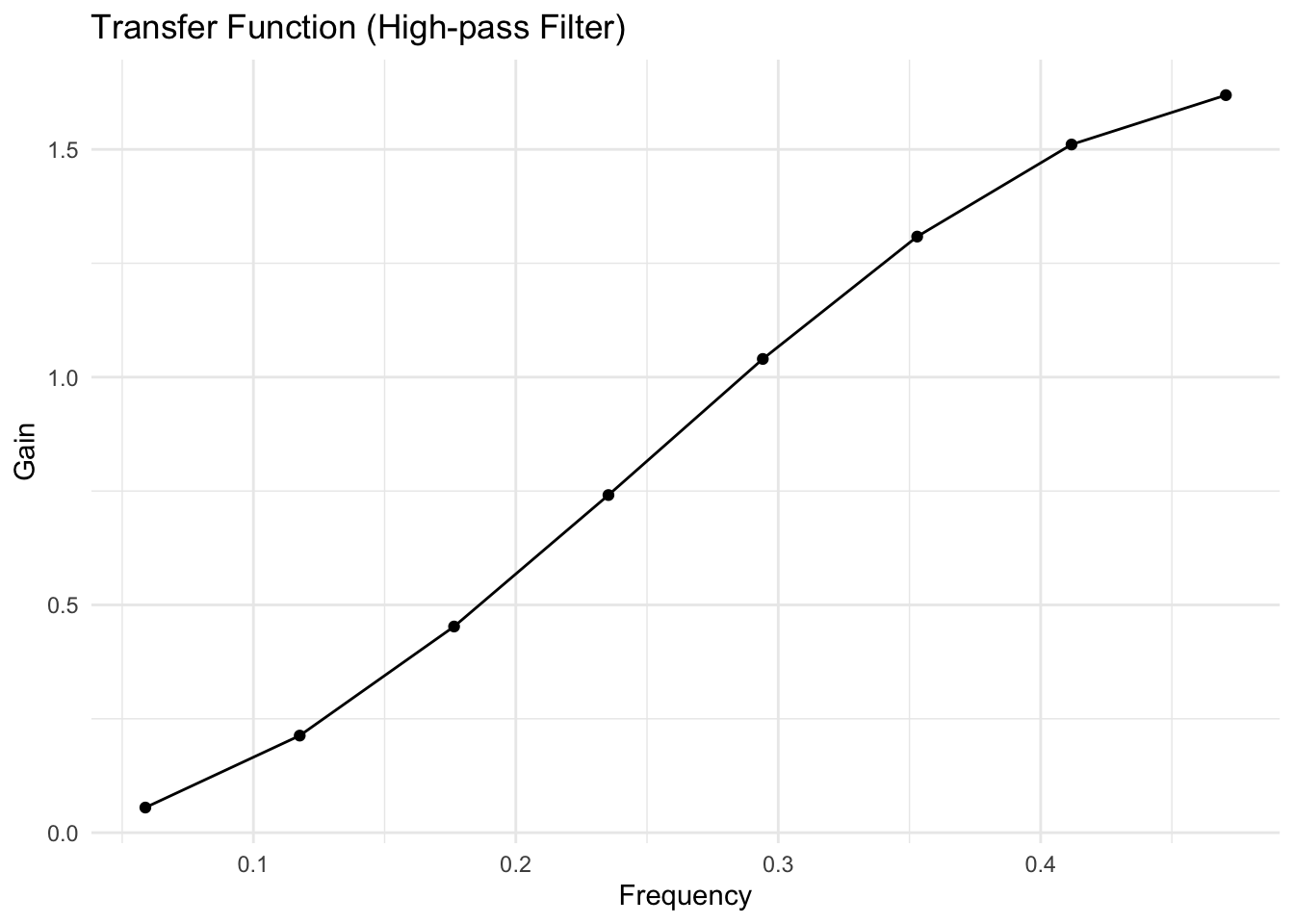
Below is the transfer function corresponding to the linear filter shown previously. Here, it is clear that the higher frequencies (near \(f=1/2\)) are given greater weight than the lower frequencies.

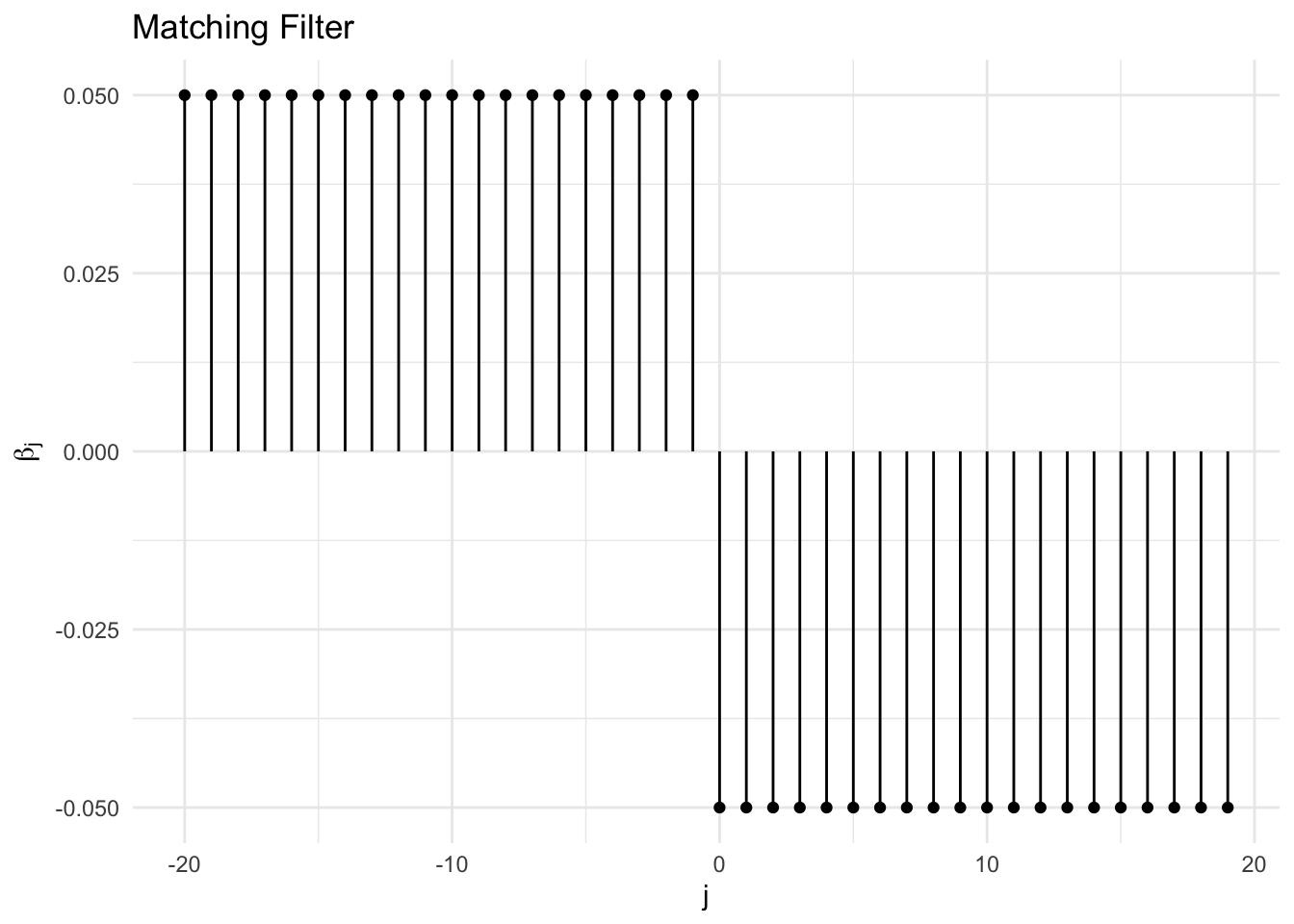
4.2.4 Matching Filter

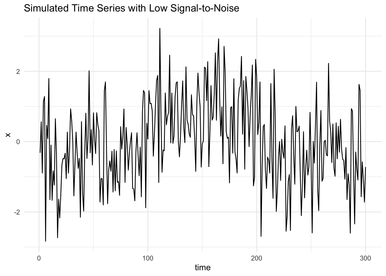
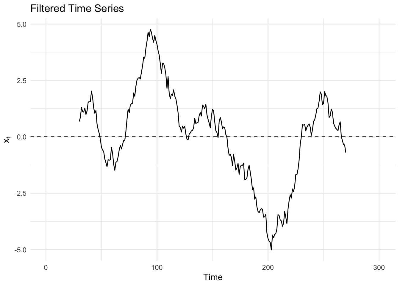
The simulated series below is an example of a time series that has a clear jump at a specific point in time.

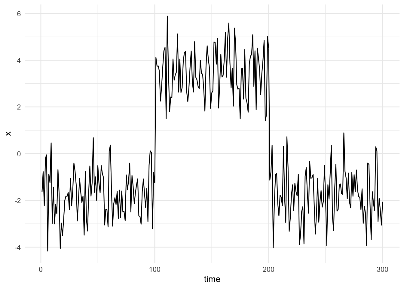
In some applications, it is desired to identify when the jump takes place in the series. We can do that by using a matching filter, which mirrors the jump in the data.

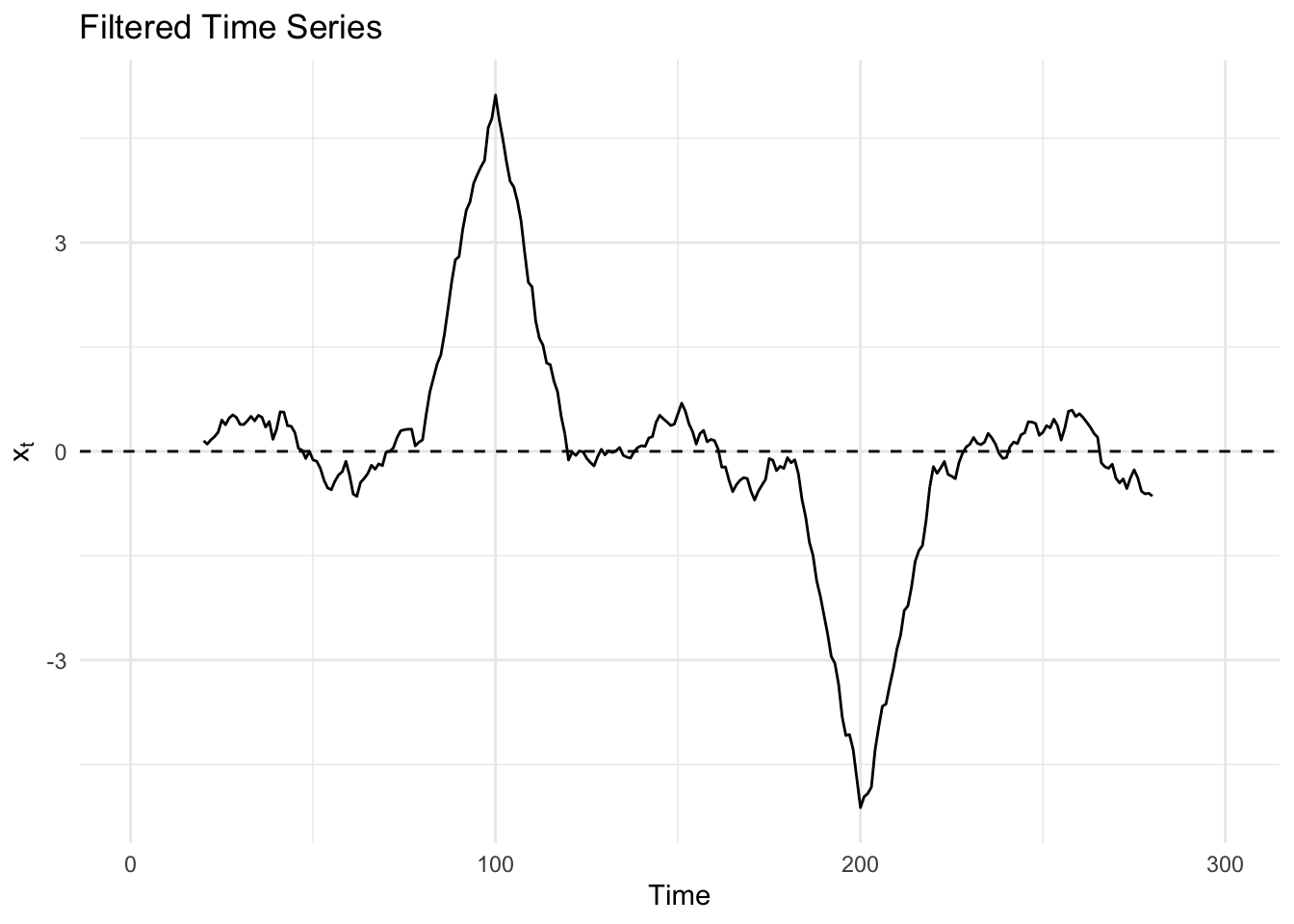
Convolving the matching filter with the data gives us the following output. We can see that the filtered series goes very high at the jump point and similarly goes very negative when the data jump back down.

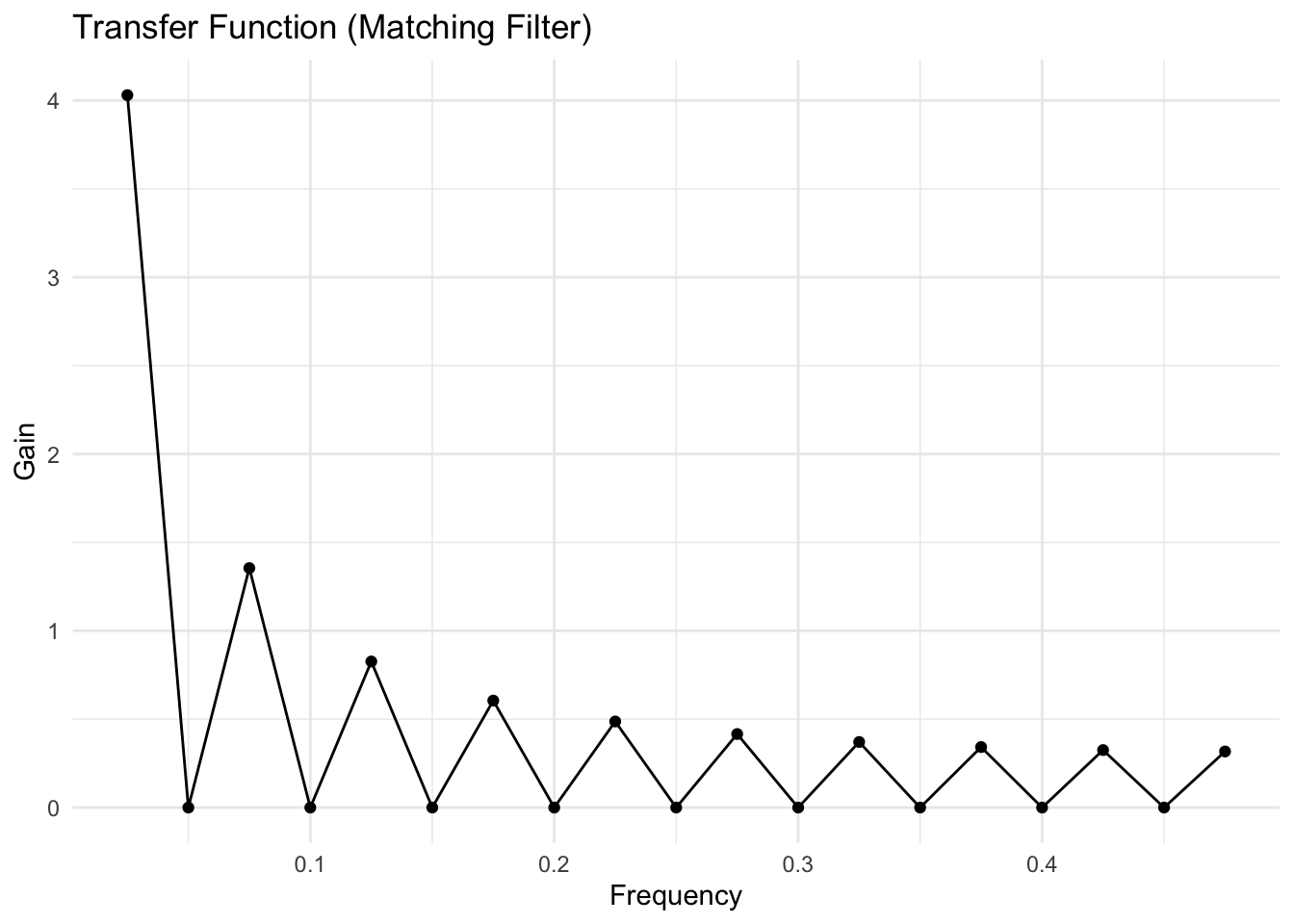
The transfer function for the matching filter is shown below. We can see that the sines and cosines in the Fourier transform have a difficult time approximating the discontinuous nature of this linear filter. Hence, the oscillation in the transfer function.

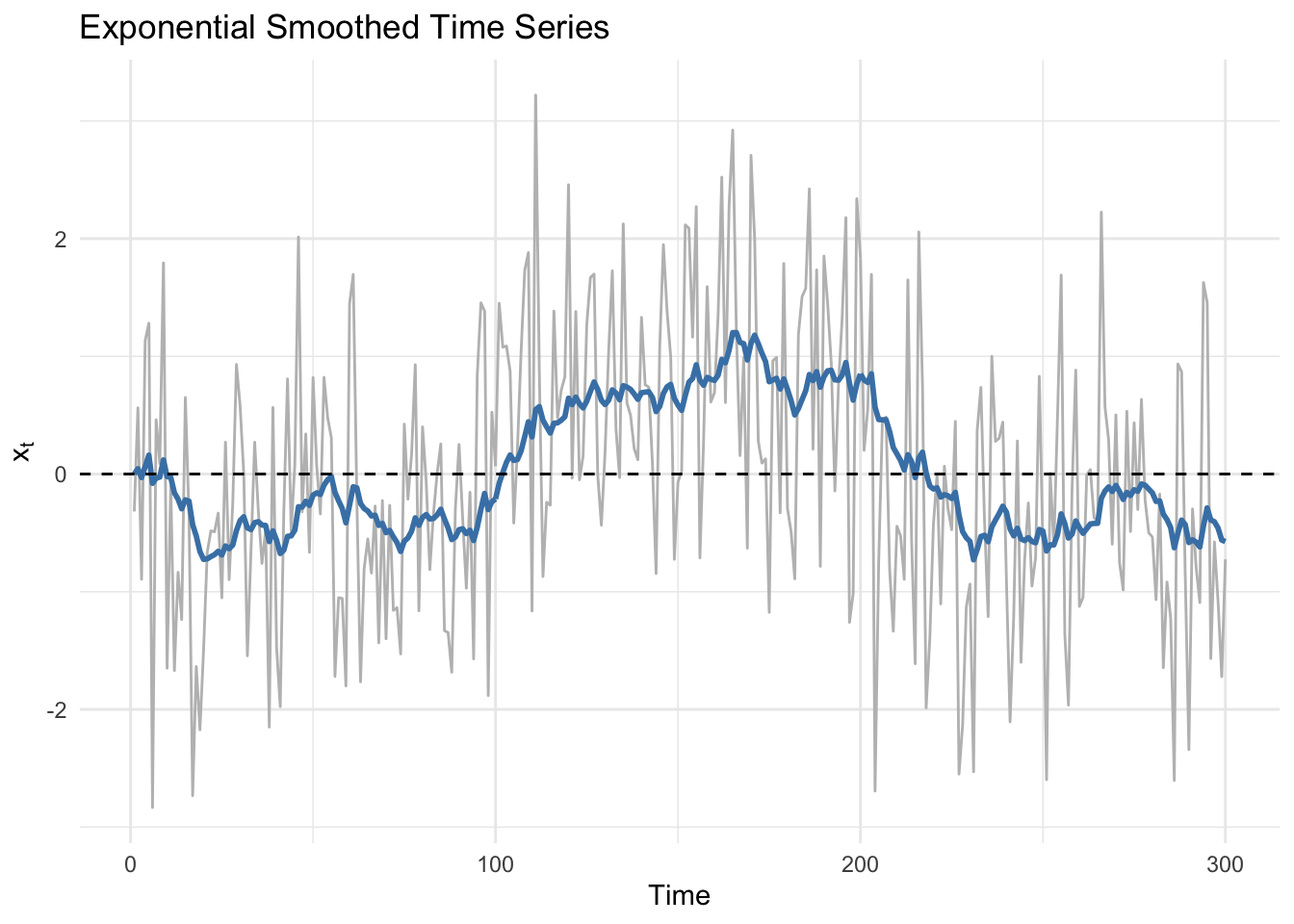
4.2.5 Exponential Smoother

\[\begin{eqnarray*} y_{t+1} & = & (1-\lambda)\sum_{j=0}^\infty\lambda^j x_{t-j}\\ & = & (1-\lambda)x_t + \lambda y_t \end{eqnarray*}\]