2.1 Example: Air Pollution and Health
For example, we may be interested in studying how long-term exposure to ambient air pollution affects your life expectancy. For example, some studies have suggested that living in a more polluted city all your life can decrease your life expectancy by as much as 6 months relative to living in a cleaner city. When thinking about how to address this problem and how one might analyze the data, we are primarily interested in comparing long-term average pollution levels between cities, perhaps over a period of decades. We are not likely to care how high the level of pollution was on a given day, or even month.
On the other hand, numerous studies have suggested that short-term spikes in air pollution can increase the number of deaths and hospitalizations in a city for cardiovascular and respiratory diseases. In this kind of situation, we may be interested in comparing day-to-day variation in air pollution to day-to-day changes in hospitalizations or mortality. The overall long-term average level of pollution is of little interest.
Consider the following time series plot of particulate matter (PM10) data from Detroit, Michigan over the period 1987–1999.
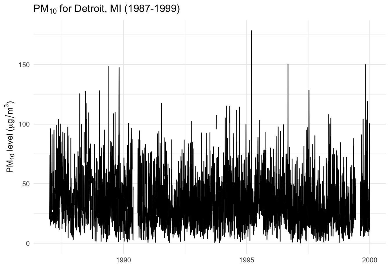
One might ask a seemingly simple question: Has air pollution in Detroit improved over the period 1987–1999? There is in fact a small but persistent overall decrease in pollution levels over this time period.

Indeed, when we look at the fitted simple linear regression model results we see that the coefficient for the slope is negative.
# A tibble: 2 x 5
  term        estimate std.error statistic   p.value
  <chr>          <dbl>     <dbl>     <dbl>     <dbl>
1 (Intercept) 48.4      1.67         28.9  9.59e-170
2 date        -0.00157  0.000184     -8.54 1.77e- 17
However, when looking at the plot above it’s difficult not to notice the extreme spikes that occur on a regular basis. A cursory reading of the plot shows days where the levels of PM10 reach over 100 \(\mu\)g/m\(^3\). So PM10 in Detroit is decreasing over time but we still experience high levels on certain days. Are things improving or not?
The answer, of course, has to do with the time scale at which we consider the data. Over a long-term time scales it looks like things are decreasing, hence the smooth trend. However, over short-term time scales, we still see large spikes. There is no one answer; the answer depends on the time scale.
From a policy perspective, we may employ different strategies to affect air pollution over long-term vs. short-term time scales. To change pollution levels over the long-term, we may attempt to convert the local economy from fossil fuel-based sources of energy to more renewable, less polluting sources. Such a plan could have a big impact but would take significant time to implement. To address short-term fluctuations in pollution, we might implement policies like traffic bans or targeted source-based interventions to mitigate short-term spikes.
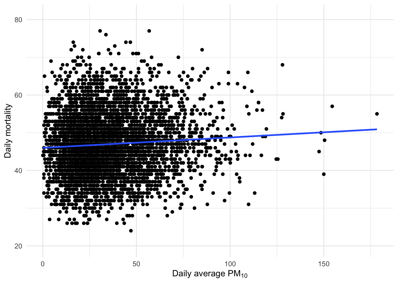
Now suppose we want to see if there is any association between mortality and air pollution in Detroit. We can make a simple scatterplot to see if there is a simple association.
Now, this scatterplot is what we might make if we did not have time series data. However, because we do have time series data, we should immediately start thinking about things in terms of different time scales of variation. Do we care about long-term associations between pollution and mortality or do we care about short-term associations?
The overall association shown in the plot above can be quantified with a simple linear regression model.
# A tibble: 2 x 5
  term        estimate std.error statistic    p.value
  <chr>          <dbl>     <dbl>     <dbl>      <dbl>
1 (Intercept)  46.0      0.226      204.   0
2 pm10          0.0275   0.00564      4.88 0.00000108
There appears to be a positive association between the two, suggesting increases in air pollution levels are associated with increases in mortality. But can we do more to gain more insight?
Let’s compute the annual mean of PM10 and sum the annual total number of deaths and make a scatter plot of these annual summary statistics.
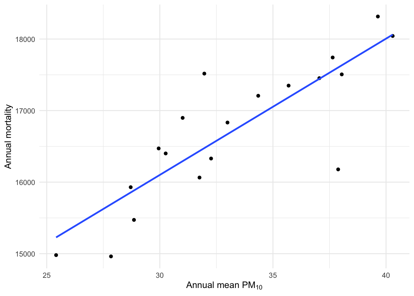
We can see from this plot the association appears quite strong (of course, there are only 13 data points). When we fit a linear model to these data, we get the following.
# A tibble: 2 x 5
  term        estimate std.error statistic       p.value
  <chr>          <dbl>     <dbl>     <dbl>         <dbl>
1 (Intercept)   10388.     987.      10.5  0.00000000725
2 pm10            190.      29.4      6.47 0.00000579
A one-unit change in annual average PM10 from one year to the next is associated with a change of 190.4 deaths.
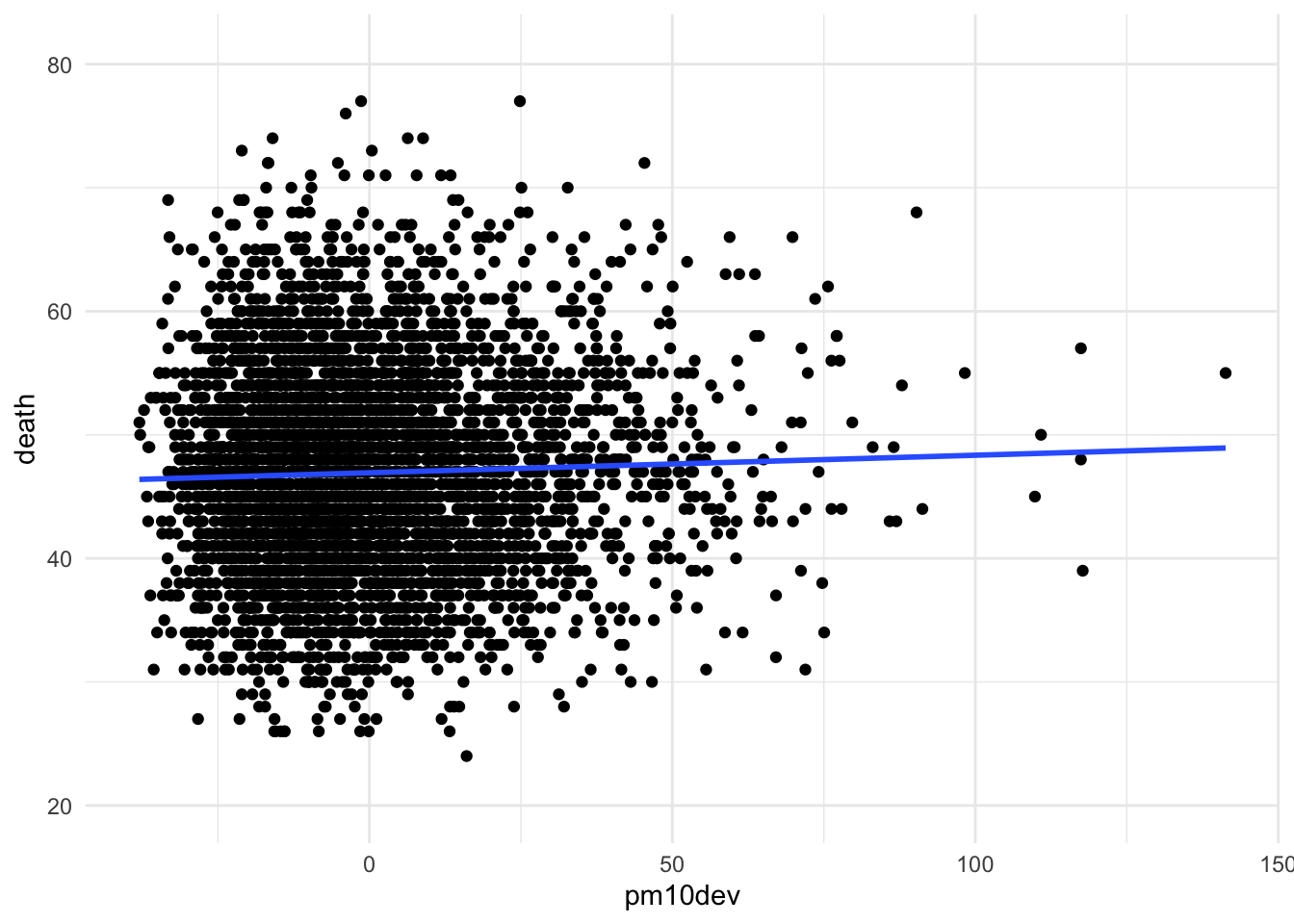
We can now take the daily deviation of PM10 from its annual mean and look at what is the association between that deviation and daily mortality.
# A tibble: 2 x 5
  term        estimate std.error statistic p.value
  <chr>          <dbl>     <dbl>     <dbl>   <dbl>
1 (Intercept)  46.9      0.116      404.    0
2 pm10dev       0.0142   0.00574      2.47  0.0136
Here the association is quite a bit smaller, but of course we are only looking at daily changes in PM10 rather than annual changes. We would not expect massive numbers of deaths associated with a one-unit change in PM10 from one day to the next.
One might be tempted to wonder: Which estimate is correct? Is it the association between daily average PM10 and mortality, or the association between yearly average PM10 and mortality? The answer is that both are “correct”, but each answers a different question. The daily average looks at short-term changes and could prehaps be interpreted as representing “acute” effects of pollution, while the yearly average might represet “chronic” effects of air pollution levels.
Another issue to consider when looking at associations at different time scales is what are the confounders that exist on this time scale? When looking at year to year changes in PM10, there are potentially many confounders that also vary across years that are associated with both PM10 and mortality. When looking at daily changes in PM10, the same confounders that vary smoothly from year to year are likely not going to be of concern. But then there might be other confounders that vary from day to day that will need to be considered.