7.1 Stationary Poisson Process

The stochastic process $N$ is a stationary Poisson process if the following hold:

For any set $A$, $N(A)$ has a Poisson distribution with mean proportional to $\|A\|$
For non-overlapping sets $A$ and $B$, $N(A)$ and $N(B)$ are independent random variables
For any set $A$, the distribution of $N(A)$ does not depend on time itself, only on the size of $A$ (i.e. stationarity)

Stationarity in the point process world is similar to stationarity in the time series world. There is a “strong” version and a “weak” or “crude” version. the strong version is as follows.

For any positive integer $r$ greater than zero and any collection of bounded sets $A_1,\dots,A_r$, we have

\[ (N(A_1),\dots,N(A_r)\stackrel{D}{=}(N(A_1+h),\dots,N(A_r+h)) \]

any $h\in\mathbb{R}$. Here, the notation $A_j+h$ has the meaning of shifting (or translating) the set $A_j$ along the real line by an amount $h$. Like with time series, this property holds for $r=1$, so that $N(A)=N(A+h)$ and so the distribution of the number of events in a set like $A$ is the same everywhere along the line. There cannot be a trend or other predictable pattern in the events.

The weaker version of stationarity says simply that for every $h$,

\[ \mathbb{P}(N(t,t+h] = k) = g(h) \]

for some function $g$. In other words, the probability density for the number of points in an interval of size $h$ only depends on $h$ (and not on $t$).

Another important property of point processes that we will generally assume is that the point process is simple. A simple point process as the feature that

\[ \mathbb{P}(N(\{t\}) =\text{$0$ or $1$ for all $t$}) = 1. \]

In other words, you cannot have more than one point that occurs at any given time. While it is generally reasonable to assume this to be true, coarseness in measurement technology might force us to measure to events as occurring at the same time in a given dataset. In such cases, it is usually possible to either ignore the duplicate event or to use the number of events occuring at a given time as a kind of covariate, also known as a “mark” in the point process literature. We will not consider here and from now on will assume that all point processes are simple.

Finally, using the notation we have here of $N(0,t]$ representing the cumulative number of points up to and including time $t$, a point process then can be thought of as a non-decreasing, right continuous, and integer-valued step function.

Another characterization of the Poisson process is via the inter-event times $u_i = t_i-t_{i-1}$. For a stationary Poisson process of rate $\lambda$, the inter-event times $u_1,\dots,u_n$ are iid exponentially distributed random variables with mean $1/\lambda$.

7.1.1 Connection to Survival Analysis

Point process models are sometimes discussed in the context of survival analysis. Survival analysis is to point process analysis much like longitudinal data analysis is to time series analysis. In survival analysis we observe point events, but usually the points represent a terminal event (“death”) and so we do not observe more than one. However, we typically observe many subjects, so in that way we observe many points across many subjects.

The kinds of point process data we will be discussing here will generally consist of many points occurring over a long time line. Much like with time series analysis, we will generally only observe a single realization and will rely on stationarity and ergodicity (i.e. mixing) to make inference from the data.

7.1.2 Connection to Time Series Analysis

As noted above, often measurement technology is such that we are not able to measure the occurrence of events in “continuous” time, but rather in some coarser discrete time. Therefore, it can be a bit of a judgment call as to whether we treat the data as point process data or not. Depending on how frequent the events are, it may be more reasonable to bin the timeline into equally spaced bins and treat the number of events in each bin as a count time series. If the events are very rare, this may end up being a binary time series. However, in that case it may make sense to simply model the data as a point process anyway.

One disadvantage to modeling point process data as count time series is that within each bin, you lose the time ordering aspect of the data because past an future mix together within the bin. Therefore, you cannot make predictions of the “next event” using such models because you cannot build a model that is conditional on only the history of the process.

7.1.3 Example: Southern California Earthquakes

The plot below shows the times and magnitudes of a collection of earthquakes occurring in the Southern California region in January 2019.

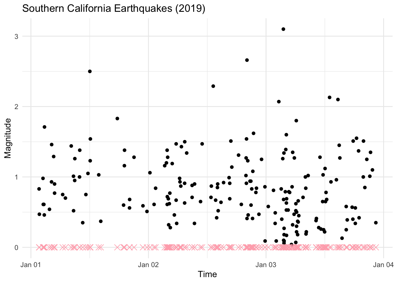
The “x”s on the x-axis mark the times of occurrence of each earthquake. These “x”s are the points of the point process and it may be our goal to predict when an earthquake might occur based on the history of earthquakes up until this point.

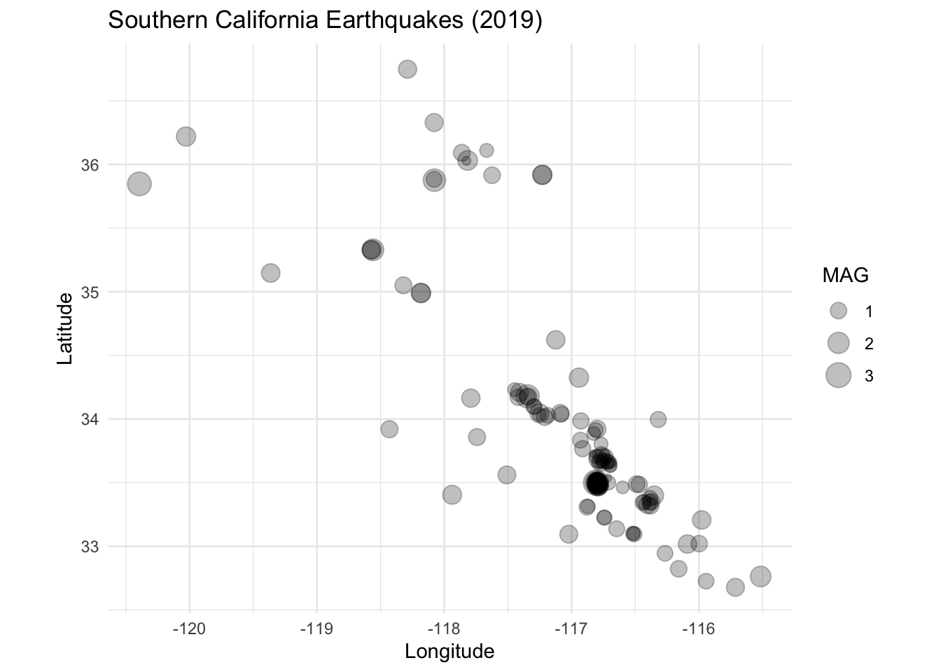
Here is a map of the earthquake locations.

A nonparametric way to describe the point process data here would be to make a histogram of the points. Here, we set the bin size of the histogram to be 3 hours. Again, the events are marked by “x”s.

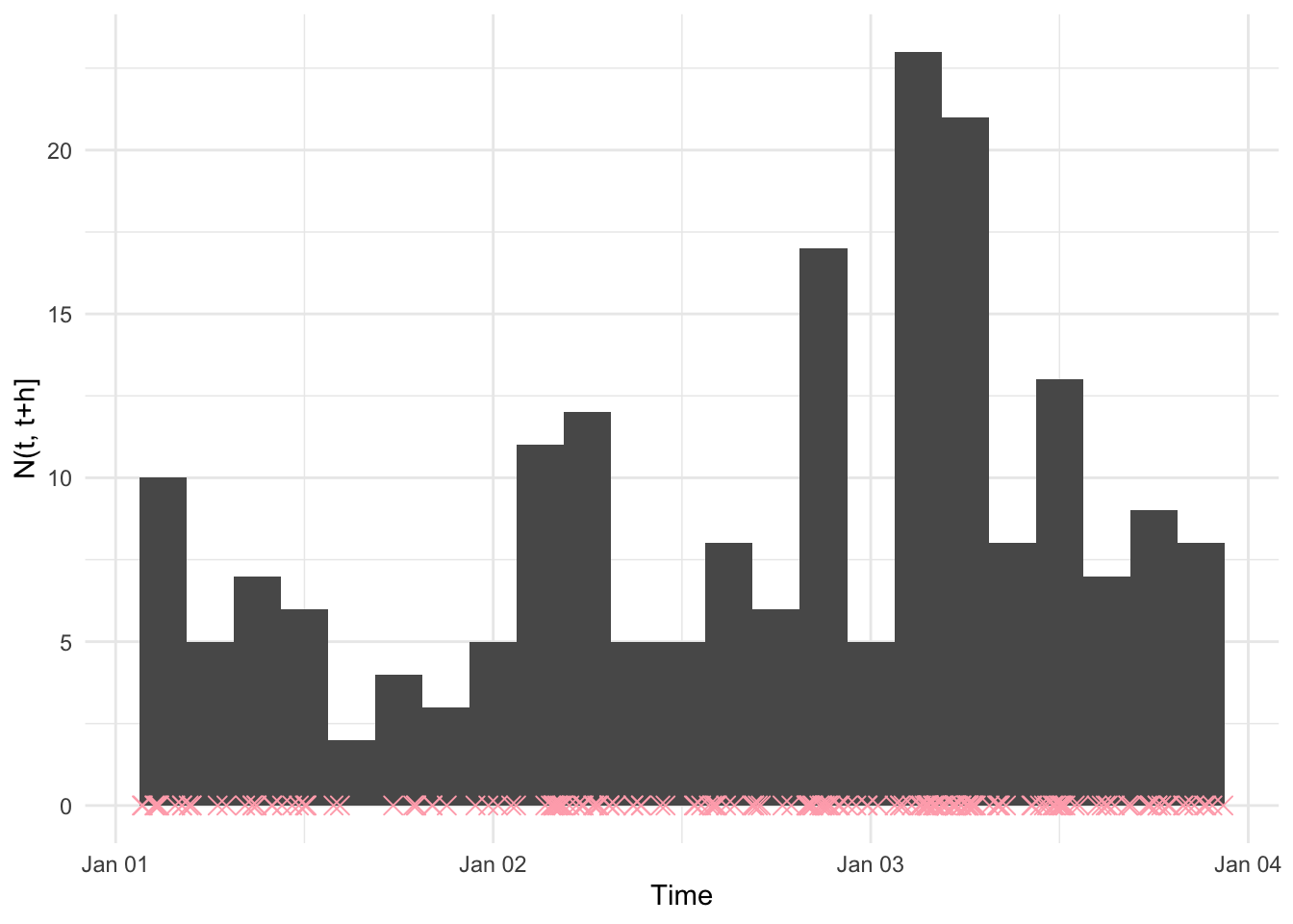
Thie histogram clearly shows the lull in events in the middle of the day on January 1st, and then an increase in frequency as we go from left to right.

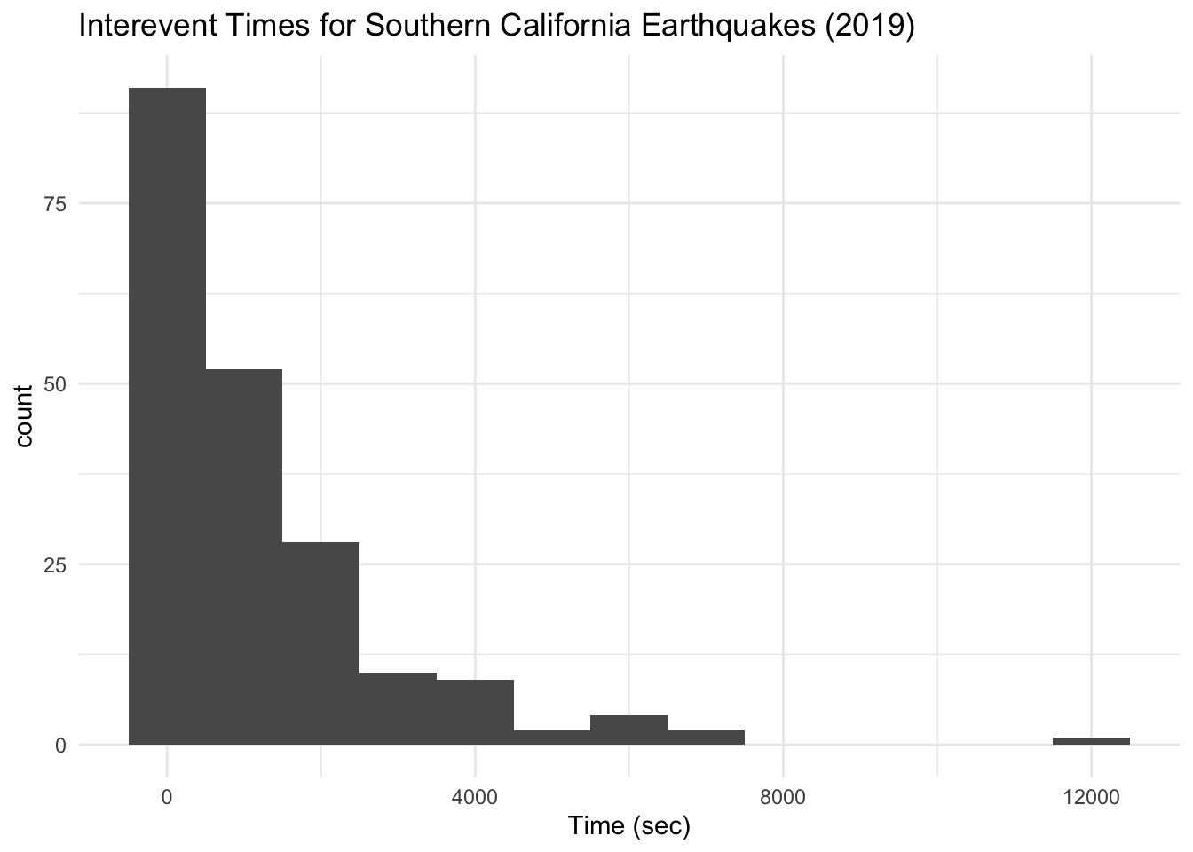
Another way to characterize point process data is not with the points themselves but rather with the intervals between the points. Seeing as the points are randomly placed on the line, the lengths of the intervals are similarly random. We can compute the observed inter-event times and make a histogram of them.

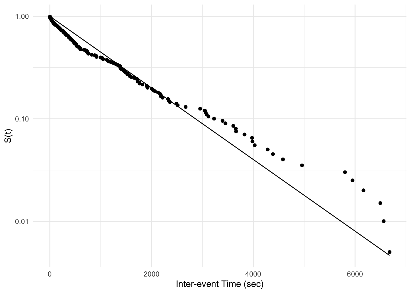
Below is a plot of the survivor function of the inter-event time distribution for the earthquake occurrences. Overlaid is the survivor function for the exponential distribution, which corresponds to a stationary Poisson process.

While a histogram can be quite useful for describing a given dataset, the are not as useful for other things we may want to do. These include

Testing specific hypotheses about the structure of earthquake occurrences
Making predictions about when the next earthquake will occur
Separating out “main shock” from “aftershock” earthquakes
Simulating earthquake realizations

For these activities, we will need a model for the conditional intensity of the point process, which we discuss below.