2.2 Fixed vs. Random Variation
Most time series books tend to imagine a time series as consisting only of random phenomena rather than as a mixture of fixed and random phenomena. As a result, the modeling is typically focused on the random aspects of time series models. However, many real time series in the world are composed of what we might think of as fixed and random variation.
Temperature data have a diurnal and seasonal component that is not “random”
Air pollution data might have day-of-week effects based on traffic or commuting patterns
While is sometimes tempting to treat everything as random, often that is a crutch that is used when we lack observations about the true underlying phenomena. Also, treating something as random when it is fixed will result in a violation of the stationarity assumption that we usually make (see below).
Depending on the nature of your application, it may make sense to model the same exact phenomena as fixed or random. In other words, it depends.
In biomedical and public health applications, we typically deal with fully observed datasets and are trying to explain “what happened?”
We are describing the past and maybe making an inference about the future
In finance or control-system applications, we may be making forecasts about future events based on the past. Things that appear fixed from the past data may change in the future and so we may want to allow for models to “adapt” to unknown future patterns.
Consider the following plot of daily average temperature in Baltimore, MD for the years 1990–1992. As one might expect from temperature data, there is a strong seasonal pattern which peaks in the summer and troughs in the winter.
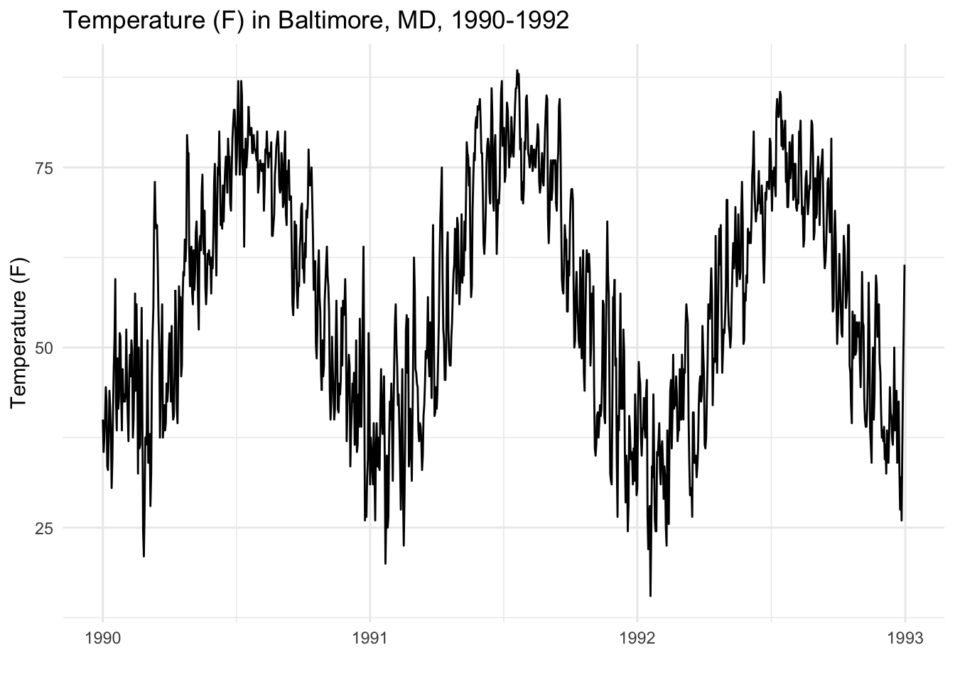
Now is this so-called seasonal pattern fixed or random? History would tell us that the seasonal pattern is fairly predictable. We generally not believe that it can freezing cold in the summer nor that it can be 90 degrees (F) in the winter.
A more formal way to discuss this might be with the following model. Let \(y_1, y_2, \dots\) be the temperature values for each day \(t\) in Baltimore and consider the following model,
\[ y_t = \mu + \varepsilon_t, \]
where \(\varepsilon\) is the random deviation between the expected value \(\mu\) and the observed value \(y_t\). Without the aid of any computer, we might look at the plot above and estimate that \(\mu\) is around 50–55 degrees. But now, imagine that your job is to predict the value of \(\varepsilon_t\) for any value of \(t\). It’s clear that if \(t\) falls during the middle of year, it’s very likely that \(\varepsilon_t > 0\) and that if \(t\) falls near the beginning or end of the year then it’s likely that \(\varepsilon_t < 0\). So there is significant information about the deviation \(\varepsilon\) that we gain simply by knowing the value of \(t\). In other words, there is a fixed seasonal effect embedded in the series \(\varepsilon_t\) which we might be hard-pressed to consider as “random”.
But now consider the following model.
\[ y_t = y_{t-1} + \varepsilon_t. \]
This model predicts the value of \(y_t\) as a deviation from the value at time \(t-1\). So today’s value is equal to yesterday’s value plus a small deviation. Now, suppose it’s your job to predict values of \(\varepsilon_t\). It’s a little bit harder, right? If I know that yesterday it was 70 degrees, do I know for sure that today will be warmer than 70? Or colder? If I know that yesterday was 20 degrees, do I know for sure that it will be warmer or colder today? In this model the deviations \(\varepsilon_t\) might seem more “random” or harder to predict. There isn’t a fixed rule that says that today’s temperature is always warmer (or colder) than yesterday’s temperature.
Consider a different time series below, which shows the weighted-mid trading price for the exchange traded fund with ticker symbol SPY. This fund tracks the S&P 500 index of U.S. stocks. Note that the time scale on the x-axis is in microseconds.
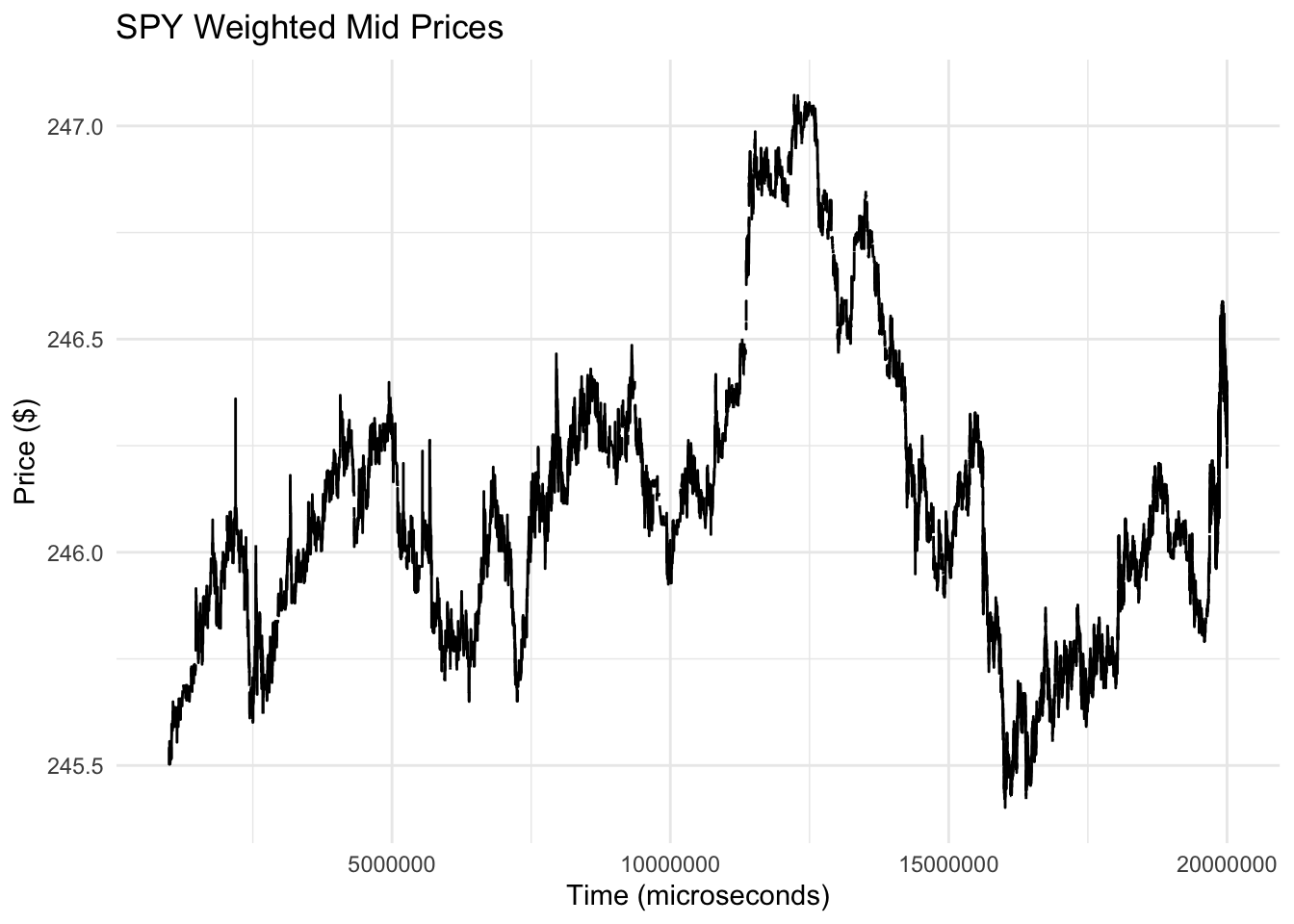
Compared to the temperature time series this plot looks a lot less regular and has no discernable pattern. Also, at the microsecond level, we may be less familiar with what fixed patterns may exist for this kind of stock price. It may be the experienced traders know that at a given time of day within a window of a few hundred thousand microseconds, that this pattern always emerges.
However, with finance, there is a theory known as the efficient markets hypothesis that states that such fixed patterns shouldn’t exist. If such a fixed pattenr existed, it would represent an arbitrage opportunity, or an opportunity to make money without risk. For example, in the plot above, we could buy the stock at time 2.5 million microseconds and then sell it later around 12.5 million microseconds for an easy profit. If this pattern existed every day, we could just tell our brokers to execute this trade every day for a small profit. However, as word of this pattern leaked out into the marketplace, more and more people would start buying at the same time as me and selling at the same time as me. This would raise the price at the time of buying and lower the price at the selling time, and eventually the profit opportunity would go away.
The efficient markets hypothesis suggest that the presence of such fixed patterns is highly unlikely. As a result, it probably makes more sense to model such data as random rather than as fixed. This suggests a different modeling strategy and different types of models that may be employed. We will not be discussing these types of models in great detail here.