4.5 Residual Autocorrelation

Suppose we fit the model

\[ y_t = \alpha + \sum_{j=0}^M \beta_j x_{t-j} + \boldsymbol{\gamma}^\prime\mathbf{z}_t + s(t; \lambda) + \varepsilon_t \]

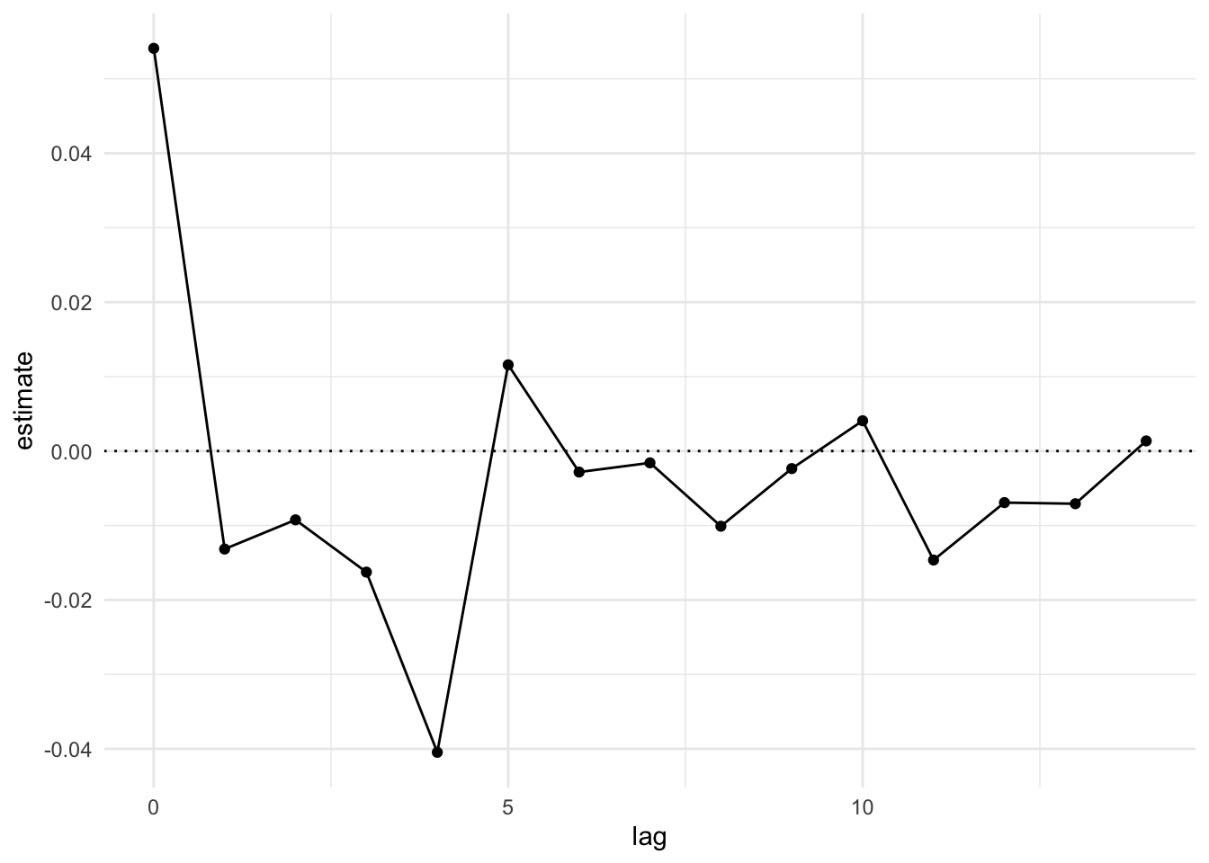
Below is a plot of the distributed lag function associated with \(x_t\).

But what about standard errors? How should we compute them?

Traditional linear models assume that

\[ \text{Var}(\varepsilon_1,\dots,\varepsilon_t) = \sigma^2I \]

As a result, if \(\boldsymbol{\theta}\) is our vector of regression model parameters, we have \[ \text{Var}(\boldsymbol{\theta}) = \sigma^2(X^\prime X)^{-1}. \]

where \(I\) is an \(n\times n\) identity matrix. However, with time series data, it’s possible that the residuals are autocorrelated. We can check this by plotting the ACF of the residuals.

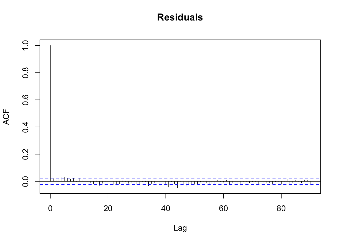
If there were substantial autocorrelation in the residuals, that would suggest the independent error model were incorrect.

The general idea to the robust approach to making inferences about \(\boldsymbol{\theta}\) works in two parts

1. Estimate the model parameters using a “working model” or “working covariance” matrix \(W^{-1}\). This can be independence or something else.

2. Compute a separate covariance matrix \(\hat{V}\) for the errors. In this case, we may use something based on an estimated autocovariance function.

Then we can compute a robust variance estimator for the model regression parameters as

\[ \text{Var}(\hat{\boldsymbol{\theta}}) = (X^\prime WX)^{-1}X^\prime W\,\hat{V}\,WX(X^\prime WX)^{-1} \]

If it turns out that \(\hat{V}=W^{-1}\), so that the working model is in fact the true model, then we have the usual least squares variance estimator.