Chapter 3 Frequency and Time Scale Analysis
Time scale analysis of time series data most directly addresses the idea that time series data represent a mixture of variation at different time scales. Frequency-based methods of analysis are designed to separate out the variation at those different time scales and to examine which scales are “interesting” in a given context. Critical to the idea of time scale analysis is Parseval’s theorem which says, roughly, that the total variation in a time series is equal to the sum of the variation across all time scales. We will discuss this in more detail later.
Consider the time series of length \(n\), \(y_0, y_1, \dots, y_t, \dots, y_{n-1}\) and for the sake of simplicity we will assume that \(n\) is even. For this chapter, we will start our \(t\) indexing from \(0\) as it simplifies some of the formulas.
As an example, we will use daily temperature data from Baltimore, MD. The data represent 24-hour average temperatures taken from a monitor in downtown Baltimore. Here is a plot of the data from 1990–1991.
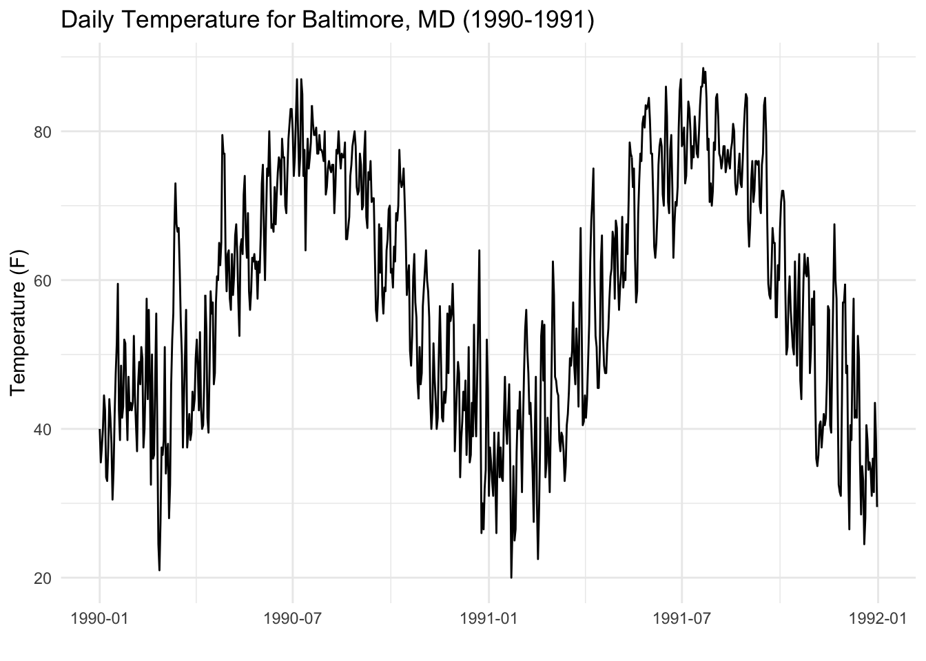
Anyone familiar with the concept of temperature should find the data completely unsurprising. However, they make for a useful dataset as our expectations about what should be in the data are fairly well-grounded.
Suppose we wanted to know if there is an annual cycle in the data. From looking at the plot, it’s clear that there is an annual cycle, but bear with me here. We might fit the following linear model:
\[ y_t = \beta_0 + \beta_1\cos(2\pi t\cdot 1 / 365) + \varepsilon_t. \]
This model fits a single cosine term with a period of exactly 365 days (i.e. the number of days in 1 year).
# A tibble: 2 x 5
  term                   estimate std.error statistic p.value
  <chr>                     <dbl>     <dbl>     <dbl>   <dbl>
1 (Intercept)                55.9     0.119      469.       0
2 cos(time * 2 * pi/365)    -19.7     0.168     -117.       0
Below is a plot of the fit for just the 1990–1991 portion of the data.
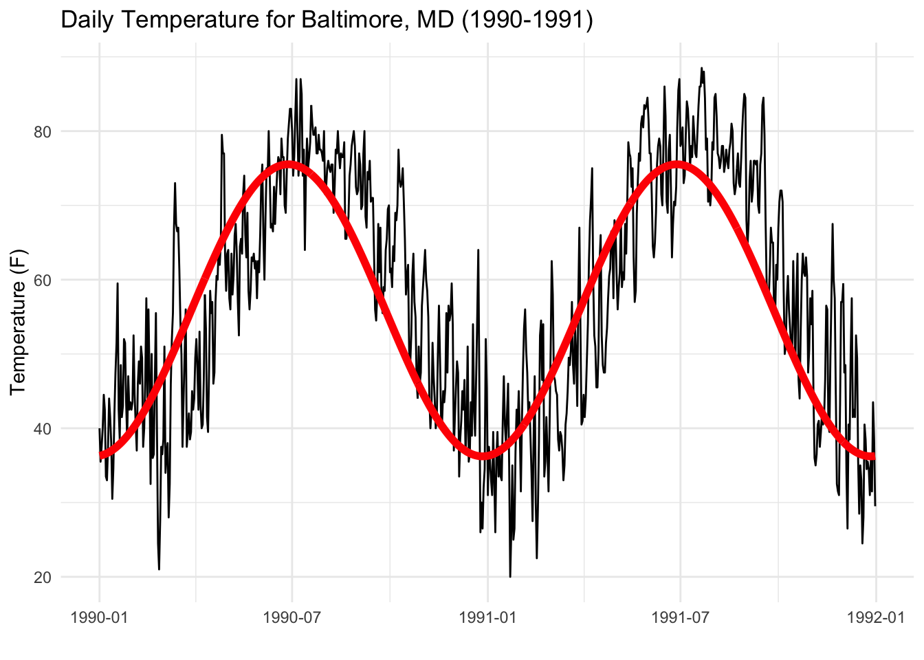
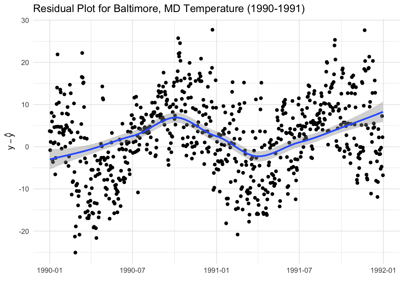
You can see that it’s not exactly a great fit, suggesting that the model is perhaps not the idea model for predicting temperature. In particular, the time plot of the residuals show some clear patterns.
But we are not exactly here to predict temperature. Rather we want to know how much variation exists at the annual (365-day) time scale. We can see from the model output above that the coefficient for the cosine term \(\beta_1\) is \(-19.7\).
How large is \(-19.7\)? It’s difficult to say without more context. It’s obviously statistically significant, as we can see from the model output, but that’s not quite enough information. To what do we compare this coefficient?
One thing we can do is try and see if there is another prominent cycle at a different frequency. For example, maybe there is a sub-annual cycle that occurs twice a year? This cycle would occur at a period of roughly 182 days (half a year). We could explore this by fitting a model like the following.
\[ y_t = \beta_0 + \beta_1\cos(2\pi t\cdot 1 / 365) + \beta_2\cos(2\pi t \cdot 2/365) + \varepsilon_t. \] This model fits two cosines, one with a 1-year period and one with a half-year period. Fitting this model to the same data gives us
# A tibble: 3 x 5
  term                       estimate std.error statistic p.value
  <chr>                         <dbl>     <dbl>     <dbl>   <dbl>
1 (Intercept)                  55.9       0.119    469.    0
2 cos(time * 2 * pi/365)      -19.7       0.168   -117.    0
3 cos(time * 2 * pi * 2/365)   -0.304     0.168     -1.80  0.0711
We can see from the model output the coefficient for the 1-year period cosine remains unchanged from the previous model fit. That is because the new cosine term that we included in the model is orthogonal to the first term. The second term in the model, the one with the half-year period, has a coefficient of \(-0.3\), which is quite a bit smaller than the estimate of \(\beta_2\). Clearly, the data places much less weight on the 182-day cycle than there is on the 365-day cycle. We can do this one more time and see whether there is a 120-day cycle in the data (i.e. 3 times per year) by fitting the model
\[ y_t = \beta_0 + \beta_1\cos(2\pi t / 365) + \beta_2\cos(2\pi t\cdot 2/365) + \beta_3\cos(2\pi t \cdot 3/365) + \varepsilon_t. \]
# A tibble: 4 x 5
  term                       estimate std.error statistic p.value
  <chr>                         <dbl>     <dbl>     <dbl>   <dbl>
1 (Intercept)                  55.9       0.119   469.     0
2 cos(time * 2 * pi/365)      -19.7       0.168  -117.     0
3 cos(time * 2 * pi * 2/365)   -0.304     0.168    -1.81   0.0709
4 cos(time * 2 * pi * 3/365)    0.163     0.168     0.966  0.334
Here, it seems like there is little evidence of a the data being correlated with a cosine that has 3 cycles per year. The estimate of \(\beta_4\) is \(0.16\), which is close to zero, especially relative to the estimate for \(\beta_1\).
We can also look at lower frequency variation, so for example, if there is a cycle that occurs once every 4 years. That can be estimated with the following model.
\[\begin{eqnarray*} y_t & = & \beta_0 + \beta_1\cos(2\pi t\cdot 1 / 365) + \beta_2\cos(2\pi t\cdot 2/365)\\ & & + \beta_3\cos(2\pi t \cdot 3/365) + \beta_4\cos(2\pi t\cdot0.25/365) + \varepsilon_t. \end{eqnarray*}\]
# A tibble: 5 x 5
  term                          estimate std.error statistic p.value
  <chr>                            <dbl>     <dbl>     <dbl>   <dbl>
1 (Intercept)                     55.9       0.119   469.    0
2 cos(time * 2 * pi/365)         -19.7       0.168  -117.    0
3 cos(time * 2 * pi * 2/365)      -0.306     0.168    -1.82  0.0690
4 cos(time * 2 * pi * 3/365)       0.161     0.168     0.957 0.338
5 cos(time * 2 * pi * 0.25/365)    0.539     0.168     3.20  0.00136
Again, the coefficient estimate for \(\beta_4\) is not particularly large, suggesting that the once-every-4-year cycle is not a dominant source of variation.
In principle, we could continue to add more cosine terms to the model (up to \(n/2\) of them) and see how the temperature data were correlated with each of them. The absolute value of the coefficient associated with each cosine term would give us a sense of how much variation is associated with a given frequency time scale. Given the nature of temperature, it appears likely that the greatest amount of variation would occur at the 1-cycle per year time scale. However, there may be hidden cycles that are difficult to see visually with the data that a more formal analysis can reveal. This is the essence of time scale analysis.