2.6 Example: Filtering an Endowment Spending Rule

University endowments are typically confronted with two conflicting goals. On the one hand, they are expected to last forever, in order to provide support for future generations of students. However, on the other hand, they are expected to provide support for current students. The former goal suggests focusing on riskier investments that promise higher long-term returns, while the latter goal suggests focusing on conservative investments that can provide stable income (but may be outpaced by inflation in the long run).

A typical university endowment has a target spending rate, which is roughly the percent of the total endowment that is withdrawn from the endowment and transferred to the university’s operating budget. Often the target rate is in the range of 4%-6% of the endowment value. Two extreme strategies are

1. Spend exactly the target rate (e.g. 4%) of the endowment every year. This strategy obviously achieves the target rate exactly but subjects the university’s operating budget to potentially wild swings of the stock and bond markets from year to year. Since the university cannot reasonably cut and raise employee salaries dramatically from year to year, such an endowment spending strategy would make it difficult to plan the budget.

2. Spend a fixed amount every year (adjusted for inflation), regardless of the endowment value. This strategy brings stability to the spending plan, but totally ignores potential gains or losses to the market value of the endowment. If the endowment were to increase, the university might miss opportunities to invest in new and exciting areas. If the endowment were to decline (such as the dramatic decline during the 2008–2009 recession in the U.S.), the university might overspend and damage the long-term health of the endowment.

One strategy that is employed by some universities (most notably, Yale’s Endowment) is the complementary filter, which is sometimes referred to as exponential smoothing. The idea here is to take a weighted average of current and past observations, incorporating new data as they come in.

Suppose \(y_1, y_2,\dots,y_{t-1}\) are the annual endowment market values until year \(t-1\) and let \(x_1, x_2, \dots, x_{t-1}\) be the annual amount that the university has spent from the endowment until year \(t-1\). The goal is to determine how much of the endowment to spend at time \(t\), i.e. what is our estimate of \(x_t\)?

The complementary filter approach essentially takes a weighted average between the two extreme approaches. Using a fixed spending rule our forecast for year \(t\) would have \(x_t^{t-1} = (1+\alpha) x_{t-1}\), where \(\alpha\) is the inflation rate, so for 2% inflation, \(\alpha = 0.02\). Once we observe the endowment market value \(y_t\) (in addition to \(y_{t-1}, y_{t-2}, \dots\)), how should we update our estimate? If \(\beta\) is the target spending rate (e.g. a 4% spending rule has \(\beta=0.04\)), then a strict spending rule would have the university spend \(\beta y_t\) at year \(t\).

The complementary filter works as follows. Given a tuning parameter \(\lambda\in(0, 1)\), \[ x_t = x_t^{t-1} + (1 - \lambda)(\beta y_t - x_t^{t-1}). \]

This approach incorporates new data \(y_t\) as they come int but also pulls those data towards the overall stability of the fixed spending rule. Clearly, if \(\lambda=0\) we simply follow the strict spending rule, whereas if \(\lambda=1\) we follow the fixed spending rule. So the complementary filter allows for both extreme spending rules, as well as many in between.

Below is a plot of how much money would be spent from the Yale Endowment if they stuck to a (hypothetical) strict spending rule of spending 4% of the market value every year. The data on the endowment’s market value are taken from the Yale Endowment’s annual reports.

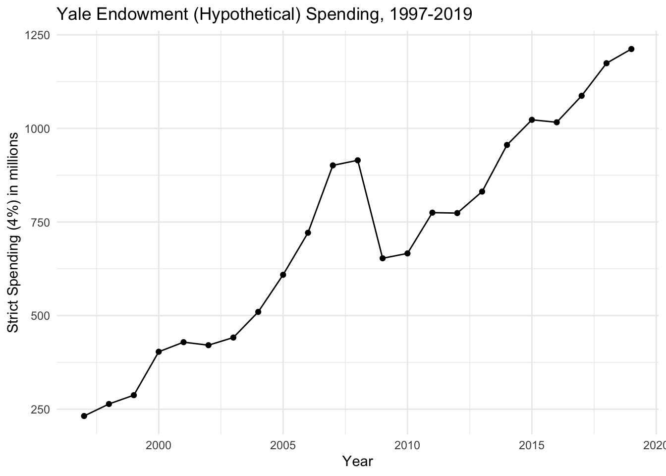
While there appears to be a general increase over the 18 year period, there is a steep drop of spending between 2008 and 2009, during which there was a severe recession. The drop is on the order of $260 million which, even for a large university like Yale, is a dramatic change from year to year. On the other hand, from 2006 to 2007, there was a sharp increase of about $180 million. Although such an increase in spending may seem beneficial, it can be difficult to responsibly incorporate such a large increase in the budget over the course of a single year.

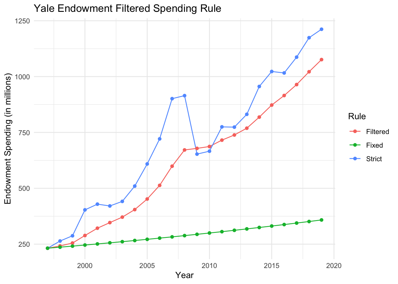
The plot above shows the spending patterns based on a stricted 4% spending rule (“Strict”), a fixed spending rule indexed to inflation (“Fixed”), and a filtered spending rule using the complementary filter with \(\lambda = 0.8\) (“Filtered”). Clearly, the filtered rule underspends relative to the endowment’s annual market value, but tracks it closer than the fixed rule and smooths out much of the variation in the market value.

The application of the complementary filter here is sometimes referred to in engineering applications as “sensor fusion”. The general idea is that we want to “fuse” two types of measurements. One comes from a fixed spending rule that is very smooth and predictable, but doesn’t adapt to market conditions. The other strictly spends according to the market value but is very noisy from year to year. The strict spending rule is in a sense less biased (because it targets the spending rule directly) but is more noisy. The fixed spending rule has essentially no noise, but over time becomes very biased.

In general, the complementary filter allows us to leverage the unbiasedness of the noisy measurements as well as the smoothness of the biased measurements. A generalization of this idea will be formulated as the Kalman filter, described in a later chapter. Another benefit of the complementary filter is that it is very simple, not requiring any complex computations beyond multiplication and addition. While this is not an issue when computations can be done on powerful computers, but is highly relevant in embedded applications where algorithms are often implemented on very small or low-capacity computers (e.g. Arduino or Raspberry Pi).