13.4 Topic Modeling
Topic modeling is a method for unsupervised classification of documents, similar to clustering on numeric data, which finds natural groups of items. Latent Dirichlet allocation (LDA) is a popular topic modeling algorithm. LDA treats each document as a mixture of topics (X% topic A, Y% topic B, etc.), and each topic as a mixture of words. Each topic is a collection of word probabilities for all of the unique words used in the corpus. LDA is implemented in the topicmodels package.
Create a topic model with the LDA function. Parameter k specifieds the number of topics. Here is an example using the AssociatedPress data set.
The tidytext package provides a tidy method for extracting the per-topic/word probabilities, called \(\beta\) from the model.
## # A tibble: 20,946 x 3
##    topic term          beta
##    <int> <chr>        <dbl>
##  1     1 percent    0.00981
##  2     2 i          0.00705
##  3     1 million    0.00684
##  4     1 new        0.00594
##  5     1 year       0.00575
##  6     2 president  0.00489
##  7     2 government 0.00452
##  8     1 billion    0.00427
##  9     2 people     0.00407
## 10     2 soviet     0.00372
## # ... with 20,936 more rows
The tidied format lends itself to plotting.
ap_topics %>%
  group_by(topic) %>%
  top_n(n = 10, wt = beta) %>%
  ungroup() %>%
  arrange(topic, -beta) %>%
  mutate(term = reorder_within(term, beta, topic)) %>%
  ggplot(aes(x = term, y = beta, fill = factor(topic))) +
  geom_col(show.legend = FALSE) +
  facet_wrap(~ topic, scales = "free") +
  coord_flip() +
  scale_x_reordered()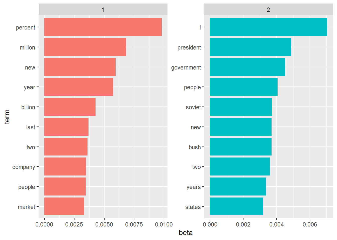
Topic 1 appears to be related to the economy; topic 2 to politics. What is the right number of topics? That’s a matter of subjectivity, but when the topics appear to be duplicative, then you’ve modeled too many topics.
Another way to look at the data is to identify terms that had the greatest difference in beta between topic 1 and topic 2. A good way to do this is with the log ratio of the two, \(log_2(\beta_2 / \beta_1)\). Log ratios are useful because the differences are symmetrical (\(log_2(2) = 1\), and \(log_2(.5) = -1\)). To constrain the analysis to a set of especially relevant words, filter for relatively common words having a beta greater than 1/1000 in at least one topic.
ap_topics %>%
  mutate(topic = paste0("topic", topic)) %>%
  pivot_wider(names_from = topic, values_from = beta) %>%
  filter(topic1 > 0.001 | topic2 > 0.001) %>%
  mutate(log_ratio = log2(topic2 / topic1)) %>%
  top_n(n = 20, w = abs(log_ratio)) %>%
  arrange(-log_ratio) %>%
  ggplot(aes(x = fct_rev(fct_inorder(term)), y = log_ratio)) +
  geom_col() +
  coord_flip()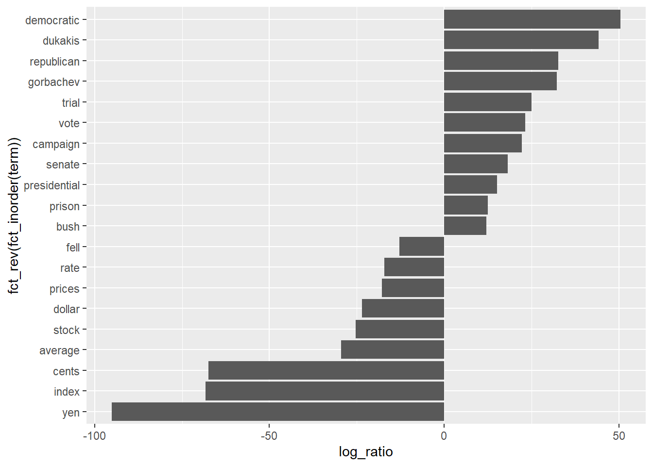
Examine the per-document-per-topic probabilities, called gamma with the matrix = "gamma" argument to tidy().
## # A tibble: 4,492 x 3
##    document topic    gamma
##       <int> <int>    <dbl>
##  1        1     1 0.248
##  2        2     1 0.362
##  3        3     1 0.527
##  4        4     1 0.357
##  5        5     1 0.181
##  6        6     1 0.000588
##  7        7     1 0.773
##  8        8     1 0.00445
##  9        9     1 0.967
## 10       10     1 0.147
## # ... with 4,482 more rows
As an example, use topic modeling to see whether the chapters for four books cluster into the right books.
library(gutenbergr)

books <- gutenberg_works(title %in% c("Twenty Thousand Leagues under the Sea",
                                      "The War of the Worlds",
                                      "Pride and Prejudice",
                                      "Great Expectations")) %>%
  gutenberg_download(meta_fields = "title")
## Warning: `filter_()` is deprecated as of dplyr 0.7.0.
## Please use `filter()` instead.
## See vignette('programming') for more help
## This warning is displayed once every 8 hours.
## Call `lifecycle::last_warnings()` to see where this warning was generated.## Determining mirror for Project Gutenberg from http://www.gutenberg.org/robot/harvest## Using mirror http://aleph.gutenberg.orgby_chapter <- books %>%
group_by(title) %>%
mutate(chapter = cumsum(str_detect(text, regex("^chapter ", ignore_case = TRUE)))) %>%
ungroup() %>%
filter(chapter > 0) %>%
unite(document, title, chapter)
by_chapter_word <- by_chapter %>%
unnest_tokens(output = word, input = text, token = "words")
word_counts <- by_chapter_word %>%
anti_join(stop_words) %>%
count(document, word, sort = TRUE) %>%
ungroup()## Joining, by = "word"## # A tibble: 104,722 x 3
## document word n
## <chr> <chr> <int>
## 1 Great Expectations_57 joe 88
## 2 Great Expectations_7 joe 70
## 3 Great Expectations_17 biddy 63
## 4 Great Expectations_27 joe 58
## 5 Great Expectations_38 estella 58
## 6 Great Expectations_2 joe 56
## 7 Great Expectations_23 pocket 53
## 8 Great Expectations_15 joe 50
## 9 Great Expectations_18 joe 50
## 10 The War of the Worlds_16 brother 50
## # ... with 104,712 more rowsThe topmodels library requires DocumentTermMatrix objects, so cast word_counts.
## <<DocumentTermMatrix (documents: 193, terms: 18215)>>
## Non-/sparse entries: 104722/3410773
## Sparsity           : 97%
## Maximal term length: 19
## Weighting          : term frequency (tf)
Create a four-topic model.
## A LDA_VEM topic model with 4 topics.What are the per-topic/word probabilities?
## # A tibble: 72,860 x 3
##    topic term        beta
##    <int> <chr>      <dbl>
##  1     1 joe     1.44e-17
##  2     2 joe     5.96e-61
##  3     3 joe     9.88e-25
##  4     4 joe     1.45e- 2
##  5     1 biddy   5.14e-28
##  6     2 biddy   5.02e-73
##  7     3 biddy   4.31e-48
##  8     4 biddy   4.78e- 3
##  9     1 estella 2.43e- 6
## 10     2 estella 4.32e-68
## # ... with 72,850 more rows
For each combination, the model computes the probability of that term being generated from that topic. The top 5 terms per topic are:
top_terms <- chapter_topics %>%
  group_by(topic) %>%
  top_n(n = 5, wt = beta) %>%
  ungroup() %>%
  arrange(topic, -beta)

top_terms %>%
  ggplot(aes(x = reorder_within(term, beta, topic), y = beta, fill = factor(topic))) +
  geom_col(show.legend = FALSE) +
  facet_wrap(~ topic, scales = "free") +
  coord_flip() +
  scale_x_reordered()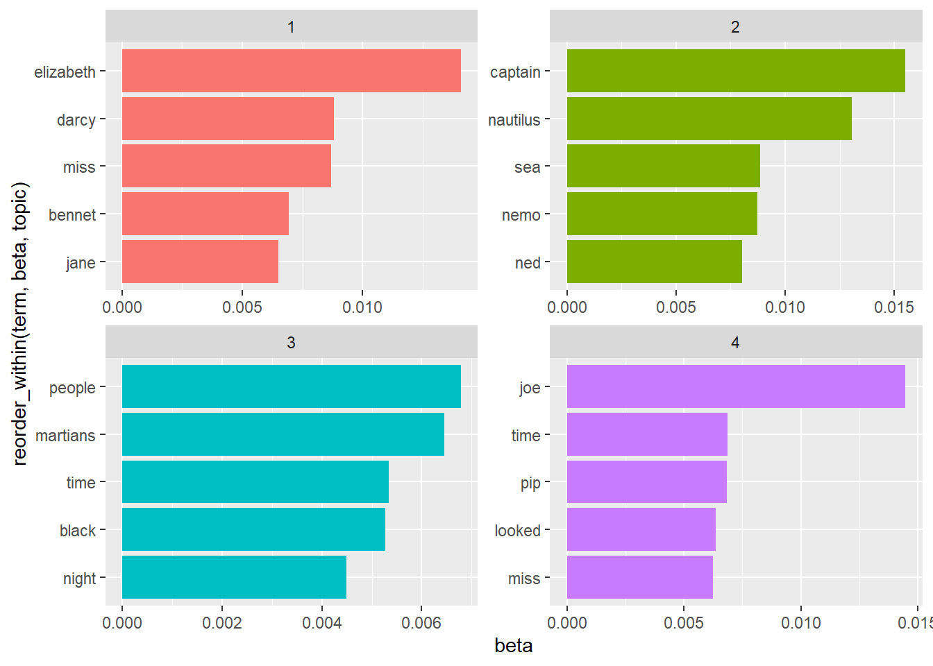
These topics are pretty clearly associated with the four books! Each “document” in this analysis was a single chapter. Which topics are associated with each document - can we put the chapters back together into the correct books? Examining the per-document-per-topic probabilities, (gamma).
Separate the document name into title and chapter, then visualize the per-document-per-topic probability for each.
chapters_gamma <- tidy(chapters_lda, matrix = "gamma") %>%
  separate(document, c("title", "chapter"), sep = "_", convert = TRUE)

chapters_gamma %>%
  mutate(title = reorder(title, gamma * topic)) %>%
  ggplot(aes(factor(topic), y = gamma)) +
  geom_boxplot() +
  facet_wrap(~ title)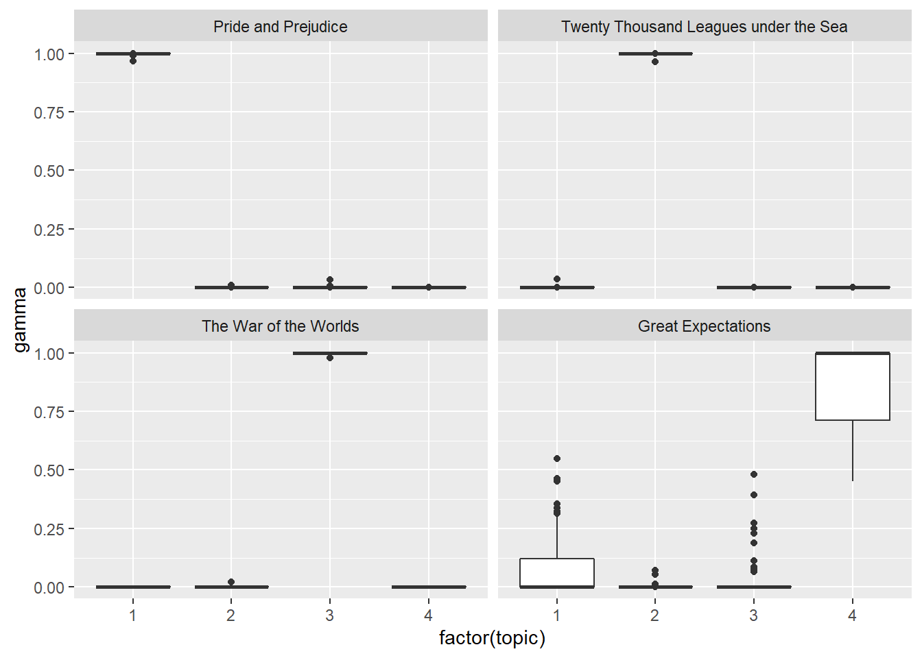
Almost all chapters from Pride and Prejudice, War of the Worlds, and Twenty Thousand Leagues Under the Sea were uniquely identified as a single topic each. Some chapters from Great Expectations (topic 4) were somewhat associated with other topics.
Are there any cases where the topic most associated with a chapter belonged to another book? First we’d find the topic that was most associated with each chapter using top_n(), which is effectively the “classification” of that chapter. We can then compare each to the “consensus” topic for each book (the most common topic among its chapters), and see which were most often misidentified.
chapter_classifications <- chapters_gamma %>%
  group_by(title, chapter) %>%
  top_n(1, gamma) %>%
  ungroup()

chapter_classifications
## # A tibble: 193 x 4
## title chapter topic gamma
## <chr> <int> <int> <dbl>
## 1 Great Expectations 23 1 0.547
## 2 Pride and Prejudice 43 1 1.00
## 3 Pride and Prejudice 18 1 1.00
## 4 Pride and Prejudice 45 1 1.00
## 5 Pride and Prejudice 16 1 1.00
## 6 Pride and Prejudice 29 1 1.00
## 7 Pride and Prejudice 10 1 1.00
## 8 Pride and Prejudice 8 1 1.00
## 9 Pride and Prejudice 56 1 1.00
## 10 Pride and Prejudice 47 1 1.00
## # ... with 183 more rowsbook_topics <- chapter_classifications %>%
count(title, topic) %>%
group_by(title) %>%
top_n(1, n) %>%
ungroup() %>%
transmute(consensus = title, topic)
chapter_classifications %>%
inner_join(book_topics, by = "topic") %>%
filter(title != consensus)## # A tibble: 2 x 5
## title chapter topic gamma consensus
## <chr> <int> <int> <dbl> <chr>
## 1 Great Expectations 23 1 0.547 Pride and Prejudice
## 2 Great Expectations 54 3 0.481 The War of the WorldsOnly two chapters from Great Expectations were misclassified.
The augment() function adds model output (token count and topic classification) to the original observations.
## # A tibble: 104,722 x 4
##    document              term  count .topic
##    <chr>                 <chr> <dbl>  <dbl>
##  1 Great Expectations_57 joe      88      4
##  2 Great Expectations_7  joe      70      4
##  3 Great Expectations_17 joe       5      4
##  4 Great Expectations_27 joe      58      4
##  5 Great Expectations_2  joe      56      4
##  6 Great Expectations_23 joe       1      4
##  7 Great Expectations_15 joe      50      4
##  8 Great Expectations_18 joe      50      4
##  9 Great Expectations_9  joe      44      4
## 10 Great Expectations_13 joe      40      4
## # ... with 104,712 more rows
Combine with the book_topics summarization to assess the misclassifications.
assignments <- assignments %>%
  separate(document, c("title", "chapter"), sep = "_", convert = TRUE) %>%
  inner_join(book_topics, by = c(".topic" = "topic"))
A good way to visualize the misclassifications is with a confusion matrix.
library(scales)

assignments %>%
  count(title, consensus, wt = count) %>%
  group_by(title) %>%
  mutate(percent = n / sum(n)) %>%
  ggplot(aes(consensus, title, fill = percent)) +
  geom_tile() +
  scale_fill_gradient2(high = "red", label = percent_format()) +
  theme_minimal() +
  theme(axis.text.x = element_text(angle = 90, hjust = 1),
        panel.grid = element_blank()) +
  labs(x = "Book words were assigned to",
       y = "Book words came from",
       fill = "% of assignments")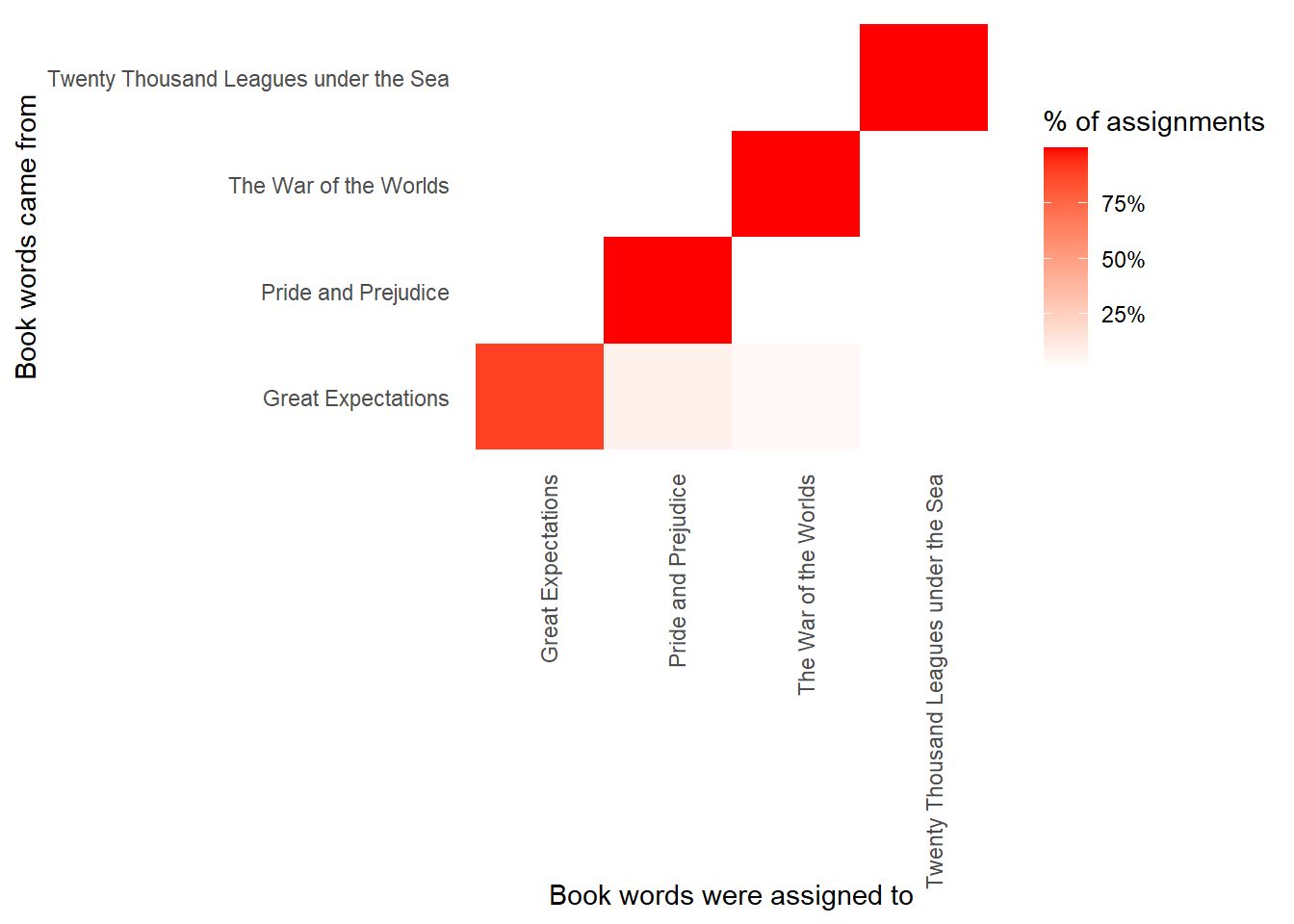
We notice that almost all the words for Pride and Prejudice, Twenty Thousand Leagues Under the Sea, and War of the Worlds were correctly assigned, while Great Expectations had a fair number of misassigned words (which, as we saw above, led to two chapters getting misclassified). What were the most commmonly mistaken words?
wrong_words <- assignments %>%
  filter(title != consensus)

wrong_words %>%
  count(title, consensus, term, wt = count) %>%
  ungroup() %>%
  arrange(desc(n))
## # A tibble: 3,551 x 4
## title consensus term n
## <chr> <chr> <chr> <dbl>
## 1 Great Expectations Pride and Prejudice love 44
## 2 Great Expectations Pride and Prejudice sergeant 37
## 3 Great Expectations Pride and Prejudice lady 32
## 4 Great Expectations Pride and Prejudice miss 26
## 5 Great Expectations The War of the Worlds boat 25
## 6 Great Expectations The War of the Worlds tide 20
## 7 Great Expectations The War of the Worlds water 20
## 8 Great Expectations Pride and Prejudice father 19
## 9 Great Expectations Pride and Prejudice baby 18
## 10 Great Expectations Pride and Prejudice flopson 18
## # ... with 3,541 more rows