Model Summary

Make predictions on the validation data set for each of the three models.

pr_ridge <- postResample(pred = predict(mdl_ridge, newdata = testing), obs = testing$mpg)
pr_lasso <- postResample(pred = predict(mdl_lasso, newdata = testing), obs = testing$mpg)
pr_elnet <- postResample(pred = predict(mdl_elnet, newdata = testing), obs = testing$mpg)

rbind(pr_ridge, pr_lasso, pr_elnet)

##          RMSE Rsquared MAE
## pr_ridge  3.7     0.90 2.8
## pr_lasso  4.0     0.97 3.0
## pr_elnet  3.7     0.90 2.8

It looks like ridge/elnet was the big winner today based on RMSE and MAE. Lasso had the best Rsquared though. On average, ridge/elnet will miss the true value of mpg by 3.75 mpg (RMSE) or 2.76 mpg (MAE). The model explains about 90% of the variation in mpg.

You can also compare the models by resampling.

model.resamples <- resamples(list(Ridge = mdl_ridge,
                                  Lasso = mdl_lasso,
                                  ELNet = mdl_elnet))
summary(model.resamples)

## 
## Call:
## summary.resamples(object = model.resamples)
## 
## Models: Ridge, Lasso, ELNet 
## Number of resamples: 25 
## 
## MAE 
##       Min. 1st Qu. Median Mean 3rd Qu. Max. NA's
## Ridge 0.66     1.6    2.2  2.1     2.5  3.5    0
## Lasso 0.81     1.9    2.2  2.3     2.6  4.0    0
## ELNet 0.66     1.6    2.2  2.1     2.5  3.5    0
## 
## RMSE 
##       Min. 1st Qu. Median Mean 3rd Qu. Max. NA's
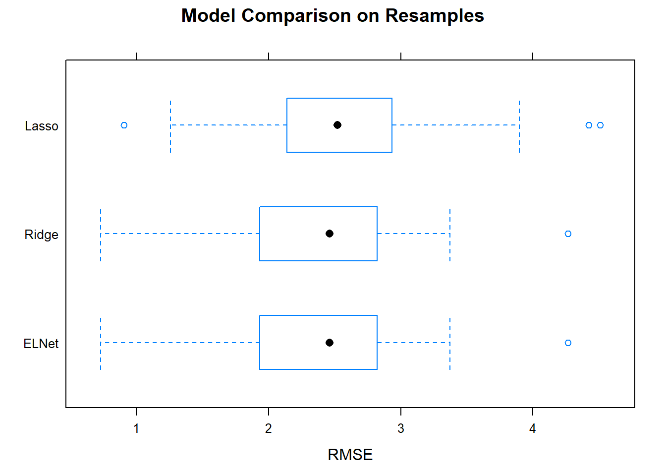
## Ridge 0.73     1.9    2.5  2.4     2.8  4.3    0
## Lasso 0.91     2.1    2.5  2.6     2.9  4.5    0
## ELNet 0.73     1.9    2.5  2.4     2.8  4.3    0
## 
## Rsquared 
##       Min. 1st Qu. Median Mean 3rd Qu. Max. NA's
## Ridge 0.69    0.84   0.89 0.88    0.94 0.98    0
## Lasso 0.63    0.81   0.87 0.86    0.94 1.00    0
## ELNet 0.69    0.84   0.89 0.88    0.94 0.98    0

You want the smallest mean RMSE, and a small range of RMSEs. Ridge/elnet had the smallest mean, and a relatively small range. Boxplots are a common way to visualize this information.

bwplot(model.resamples, metric = "RMSE", main = "Model Comparison on Resamples")

Now that you have identified the optimal model, capture its tuning parameters and refit the model to the entire data set.

set.seed(123)
mdl_final <- train(
  mpg ~ .,
  data = training,
  method = "glmnet",
  metric = "RMSE",
  preProcess = c("center", "scale"),
  tuneGrid = data.frame(
    .alpha = mdl_ridge$bestTune$alpha,  # optimized hyperparameters
    .lambda = mdl_ridge$bestTune$lambda),  # optimized hyperparameters
  trControl = train_control
  )
mdl_final

## glmnet 
## 
## 28 samples
## 10 predictors
## 
## Pre-processing: centered (10), scaled (10) 
## Resampling: Cross-Validated (5 fold, repeated 5 times) 
## Summary of sample sizes: 22, 22, 23, 22, 23, 23, ... 
## Resampling results:
## 
##   RMSE  Rsquared  MAE
##   2.4   0.89      2.1
## 
## Tuning parameter 'alpha' was held constant at a value of 0
## Tuning
##  parameter 'lambda' was held constant at a value of 2.8

The model is ready to predict on new data! Here are some final conclusions on the models.

• Lasso can set some coefficients to zero, thus performing variable selection.
• Lasso and Ridge address multicollinearity differently: in ridge regression, the coefficients of correlated predictors are similar; In lasso, one of the correlated predictors has a larger coefficient, while the rest are (nearly) zeroed.
• Lasso tends to do well if there are a small number of significant parameters and the others are close to zero. Ridge tends to work well if there are many large parameters of about the same value.
• In practice, you don’t know which will be best, so run cross-validation pick the best.