13.1 Tidy Text

The tidy text format is a table with one token (meaningful unit of text, such as a word) per row. The tidytext package assists with the major tasks in text analysis. A typical text analysis using tidy data principles unnests tokens with unnest_tokens(), removes unimportant “stop words” tokens anti_join(stop_words), and summarizes token counts count().

Here are four Jane Austin books from the janeaustenr. “Sense & Sensibility” acts as the baseline count, and the other books are faceted for comparison. Note the use of the “tribble” of custom stop words.

custom_stop_words <- tribble(
  ~word, ~lexicon,
  "edward", "CUSTOM",
  "frank", "CUSTOM",
  "thomas", "CUSTOM",
  "fanny", "CUSTOM",
  "anne", "CUSTOM"
)

austin_tidy <- austen_books() %>%
  group_by(book) %>%
  mutate(
    linenumber = row_number(),
    chapter = cumsum(str_detect(text, regex("^chapter [\\divxlc]", ignore_case = TRUE)))
    ) %>%
  ungroup() %>%
  unnest_tokens(output = word, input = text) %>%
  anti_join(stop_words) %>%
  anti_join(custom_stop_words)

## Joining, by = "word"
## Joining, by = "word"

austin_tidy %>%
  count(book, word) %>%
  group_by(book) %>%
  mutate(proportion = n / sum(n)) %>% 
  select(-n) %>% 
  pivot_wider(names_from = book, values_from = proportion) %>%
  pivot_longer(cols = `Pride & Prejudice`:`Persuasion`, names_to = "book", values_to = "proportion") %>%
  ggplot(aes(x = proportion, 
             y = `Sense & Sensibility`,
             color = abs(`Sense & Sensibility` - proportion))) +
  geom_abline(color = "gray40", lty = 2) +
  geom_jitter(alpha = 0.1, size = 2.5, width = 0.3, height = 0.3) +
  geom_text(aes(label = word), check_overlap = TRUE, vjust = 1.5) +
  scale_x_log10(labels = percent_format()) +
  scale_y_log10(labels = percent_format()) +
  scale_color_gradient(limits = c(0, 0.001), low = "darkslategray4", high = "gray75") +
  facet_wrap(~book, ncol = 2) +
  theme(legend.position = "none") +
  labs(y = "Sense & Sensibility", x = NULL)

## Warning: Removed 50931 rows containing missing values (geom_point).

## Warning: Removed 50931 rows containing missing values (geom_text).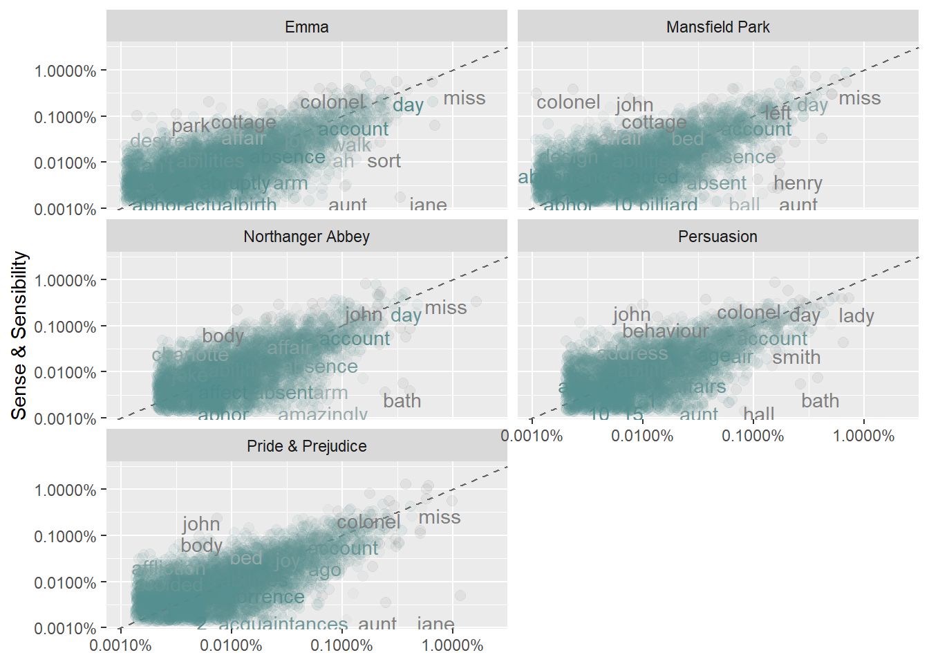

Words close to the 45-degree lines have similar frequencies in both books. Words far from the line are found more in one book more than the other. If there are few points near the low frequencies, then few infrequent words are shared. Emma is similar to Sense & Sensibility because the points are fairly narrow on the 45-degree line, and they extend all the way to the origin.

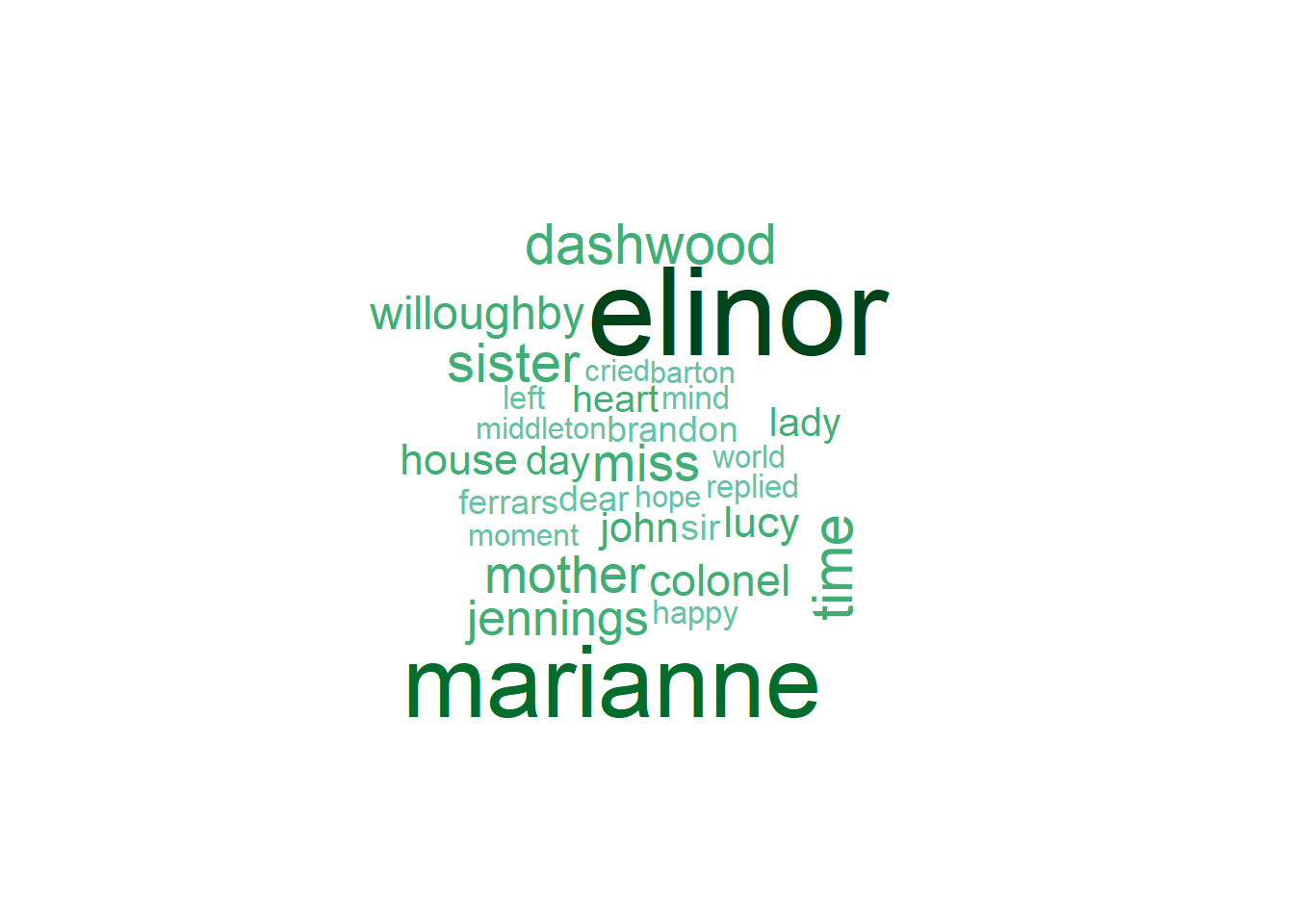
A common way to visualize words is with a word cloud. The wordcloud library is helpful. NOte that word clouds do not contain any information not already in a bar plot.

austin_word_cnt <- austin_tidy %>%
  filter(book == "Sense & Sensibility") %>%
  count(word)
pal <- brewer.pal(9,"BuGn")
pal <- pal[-(1:4)]
wordcloud(
  words = austin_word_cnt$word,
  freq = austin_word_cnt$n,
  max.words = 30,
  colors = pal
)

# pa_file <- readxl::read_excel("./../../PeoplaAnalyticsCloud.xlsx")
# pa_tidy <- pa_file %>%
#   mutate(
#     linenumber = row_number(),
#     ) %>%
#   ungroup() %>%
#   unnest_tokens(output = word, input = comment) %>%
# #  unnest_tokens(output = bigram, input = comment, token = "ngrams", n = 2) 
#   anti_join(stop_words) %>%
#   anti_join(custom_stop_words)
# pa_tidy_n <- pa_tidy %>%
#   count(word)
# pal <- brewer.pal(9,"BuGn")
# pal <- pal[-(1:4)]
# wordcloud(
#   words = pa_tidy_n$word,
#   freq = pa_tidy_n$n,
#   max.words = 30,
#   colors = pal
# )
# 
# pa_2gram <- pa_tidy %>%
#   separate(bigram, c("word1", "word2"), sep = " ") %>%
#   filter(!word1 %in% stop_words$word &
#            !word2 %in% stop_words$word &
#            !is.na(word1) & !is.na(word2)) %>%
#   unite(bigram, word1, word2, sep = " ")
# 
# 
# pa_2gram %>%
#   count(book, bigram, sort = TRUE)
# 
# pa_2gram2 <- pa_2gram %>%
#   count(bigram)
# pal <- brewer.pal(9,"BuGn")
# pal <- pal[-(1:4)]
# wordcloud(
#   words = pa_2gram2$bigram,
#   freq = pa_2gram2$n,
#   max.words = 30,
#   colors = pal
# )