7.1 Ridge
Ridge regression estimates the linear model coefficients by minimizing an augmented loss function which includes a term, \(\lambda\), that penalizes the magnitude of the coefficient estimates,
\[L = \sum_{i = 1}^n \left(y_i - x_i^{'} \hat\beta \right)^2 + \lambda \sum_{j=1}^k \hat{\beta}_j^2.\]
The resulting estimate for the coefficients is
\[\hat{\beta} = \left(X'X + \lambda I\right)^{-1}\left(X'Y \right).\]
As \(\lambda \rightarrow 0\), ridge regression approaches OLS. The bias and variance for the ridge estimator are
\[Bias(\hat{\beta}) = -\lambda \left(X'X + \lambda I \right)^{-1} \beta\] \[Var(\hat{\beta}) = \sigma^2 \left(X'X + \lambda I \right)^{-1}X'X \left(X'X + \lambda I \right)^{-1}\]
The estimator bias increases with \(\lambda\) and the estimator variance decreases with \(\lambda\). The optimal level for \(\lambda\) is the one that minimizes the root mean squared error (RMSE) or the Akaike or Bayesian Information Criterion (AIC or BIC), or R-squared.
Example
Specify alpha = 0 in a tuning grid for ridge regression (the following sections reveal how alpha distinguishes ridge, lasso, and elastic net). Note that I standardize the predictors in the preProcess step - ridge regression requires standardization.
set.seed(1234)
mdl_ridge <- train(
  mpg ~ .,
  data = training,
  method = "glmnet",
  metric = "RMSE",  # Choose from RMSE, RSquared, AIC, BIC, ...others?
  preProcess = c("center", "scale"),
  tuneGrid = expand.grid(
    .alpha = 0,  # optimize a ridge regression
    .lambda = seq(0, 5, length.out = 101)
  ),
  trControl = train_control
  )
mdl_ridge
## glmnet
##
## 28 samples
## 10 predictors
##
## Pre-processing: centered (10), scaled (10)
## Resampling: Cross-Validated (5 fold, repeated 5 times)
## Summary of sample sizes: 21, 24, 22, 21, 24, 21, ...
## Resampling results across tuning parameters:
##
## lambda RMSE Rsquared MAE
## 0.00 2.6 0.88 2.2
## 0.05 2.6 0.88 2.2
## 0.10 2.6 0.88 2.2
## 0.15 2.6 0.88 2.2
## 0.20 2.6 0.88 2.2
## 0.25 2.6 0.88 2.2
## 0.30 2.6 0.88 2.2
## 0.35 2.6 0.88 2.2
## 0.40 2.6 0.88 2.2
## 0.45 2.6 0.88 2.2
## 0.50 2.6 0.88 2.2
## 0.55 2.5 0.88 2.2
## 0.60 2.5 0.88 2.2
## 0.65 2.5 0.88 2.2
## 0.70 2.5 0.88 2.2
## 0.75 2.5 0.88 2.2
## 0.80 2.5 0.88 2.2
## 0.85 2.5 0.88 2.2
## 0.90 2.5 0.88 2.2
## 0.95 2.5 0.88 2.2
## 1.00 2.5 0.88 2.2
## 1.05 2.5 0.88 2.2
## 1.10 2.5 0.88 2.2
## 1.15 2.5 0.88 2.1
## 1.20 2.4 0.88 2.1
## 1.25 2.4 0.88 2.1
## 1.30 2.4 0.88 2.1
## 1.35 2.4 0.88 2.1
## 1.40 2.4 0.88 2.1
## 1.45 2.4 0.88 2.1
## 1.50 2.4 0.88 2.1
## 1.55 2.4 0.88 2.1
## 1.60 2.4 0.88 2.1
## 1.65 2.4 0.88 2.1
## 1.70 2.4 0.88 2.1
## 1.75 2.4 0.88 2.1
## 1.80 2.4 0.88 2.1
## 1.85 2.4 0.88 2.1
## 1.90 2.4 0.88 2.1
## 1.95 2.4 0.88 2.1
## 2.00 2.4 0.88 2.1
## 2.05 2.4 0.88 2.1
## 2.10 2.4 0.88 2.1
## 2.15 2.4 0.88 2.1
## 2.20 2.4 0.88 2.1
## 2.25 2.4 0.88 2.1
## 2.30 2.4 0.88 2.1
## 2.35 2.4 0.88 2.1
## 2.40 2.4 0.88 2.1
## 2.45 2.4 0.88 2.1
## 2.50 2.4 0.88 2.1
## 2.55 2.4 0.88 2.1
## 2.60 2.4 0.88 2.1
## 2.65 2.4 0.88 2.1
## 2.70 2.4 0.88 2.1
## 2.75 2.4 0.88 2.1
## 2.80 2.4 0.88 2.1
## 2.85 2.4 0.88 2.1
## 2.90 2.4 0.88 2.1
## 2.95 2.4 0.88 2.1
## 3.00 2.4 0.88 2.1
## 3.05 2.4 0.88 2.1
## 3.10 2.4 0.88 2.1
## 3.15 2.4 0.88 2.1
## 3.20 2.4 0.88 2.1
## 3.25 2.4 0.88 2.1
## 3.30 2.4 0.88 2.1
## 3.35 2.4 0.88 2.1
## 3.40 2.4 0.88 2.1
## 3.45 2.4 0.88 2.1
## 3.50 2.4 0.88 2.1
## 3.55 2.4 0.88 2.1
## 3.60 2.4 0.88 2.1
## 3.65 2.4 0.88 2.1
## 3.70 2.4 0.88 2.1
## 3.75 2.4 0.88 2.1
## 3.80 2.4 0.88 2.1
## 3.85 2.4 0.88 2.1
## 3.90 2.4 0.88 2.1
## 3.95 2.4 0.88 2.1
## 4.00 2.4 0.88 2.1
## 4.05 2.4 0.88 2.1
## 4.10 2.4 0.88 2.1
## 4.15 2.4 0.88 2.1
## 4.20 2.4 0.88 2.1
## 4.25 2.4 0.88 2.1
## 4.30 2.4 0.88 2.1
## 4.35 2.4 0.88 2.1
## 4.40 2.4 0.88 2.1
## 4.45 2.4 0.88 2.1
## 4.50 2.4 0.88 2.1
## 4.55 2.4 0.88 2.1
## 4.60 2.4 0.88 2.1
## 4.65 2.4 0.88 2.1
## 4.70 2.4 0.88 2.1
## 4.75 2.4 0.88 2.1
## 4.80 2.4 0.88 2.1
## 4.85 2.4 0.88 2.1
## 4.90 2.4 0.88 2.1
## 4.95 2.4 0.88 2.1
## 5.00 2.4 0.88 2.1
##
## Tuning parameter 'alpha' was held constant at a value of 0
## RMSE was used to select the optimal model using the smallest value.
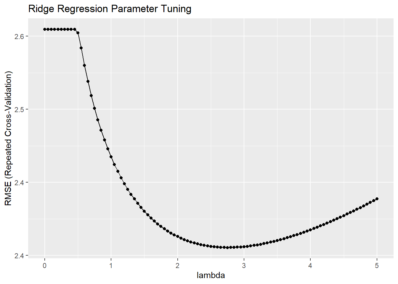
## The final values used for the model were alpha = 0 and lambda = 2.8.The model printout shows the RMSE, R-Squared, and mean absolute error (MAE) values at each lambda specified in the tuning grid. The final three lines summarize what happened. It did not tune alpha because I held it at 0 for ridge regression; it optimized using RMSE; and the optimal tuning values (at the minimum RMSE) were alpha = 0 and lambda = 2.75. You plot the model to see the tuning results.
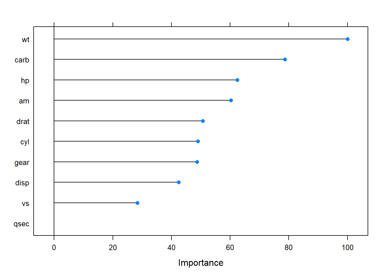
varImp() ranks the predictors by the absolute value of the coefficients in the tuned model. The most important variables here were wt, disp, and am.