13.3 Sentiment Analysis
A typical sentiment analysis involves unnesting tokens with unnest_tokens(), assigning sentiments with inner_join(sentiments), counting tokens with count(), and summarizing and visualizing.
The tidytext package contains four sentiment lexicons, all based on unigrams.
- nrc. binary “yes”/“no” for categories positive, negative, anger, anticipation, disgust, fear, joy, sadness, surprise, and trust.
- bing. “positive”/“negative” classification.
- AFINN. score between -5 (most negative) and 5 (most positive).
- loughran. “positive”/“negative”/“litigious”/“uncertainty”/“constraining”/“superflous” classification.
You can view the sentiment assignments with get_sentiments(lexicon = c("afinn", "bing", nrc", "laughlin"))
x1 <- get_sentiments(lexicon = "nrc") %>%
  count(sentiment) %>%
  mutate(lexicon = "nrc")
x2 <- get_sentiments(lexicon = "bing") %>%
  count(sentiment) %>%
  mutate(lexicon = "bing")
x3 <- get_sentiments(lexicon = "afinn") %>%
  count(value) %>%
  mutate(lexicon = "afinn") %>%
  mutate(sentiment = as.character(value)) %>%
  select(-value)
x4 <- get_sentiments(lexicon = "loughran") %>%
  count(sentiment) %>%
  mutate(lexicon = "loughran")
x <- bind_rows(x1, x2, x3, x4)

ggplot(x, aes(x = fct_reorder(sentiment, n), y = n, fill = lexicon)) +
  geom_col(show.legend = FALSE) +
  coord_flip() +
  labs(title = "Sentiment Counts", x = "", y = "") +
  facet_wrap(~ lexicon, scales = "free")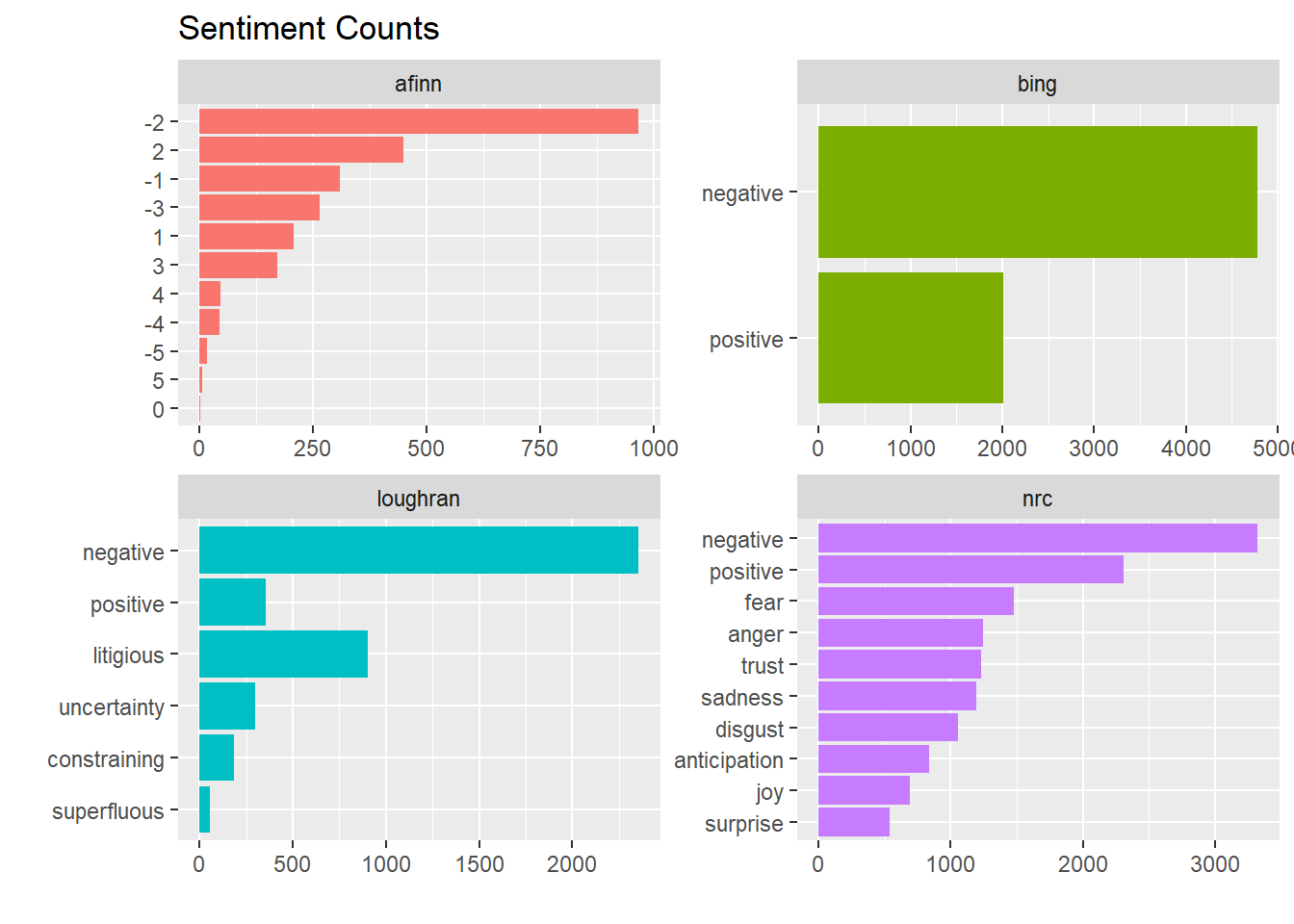
Here is a sentiment analysis of sections of 80 lines of Jane Austin’s books. (Small sections may not have enough words to get a good estimate of sentiment, and large sections can wash out the narrative structure. 80 lines seems about right.)
austin_tidy %>%
  inner_join(get_sentiments("bing")) %>%
  count(book, index = linenumber %/% 80, sentiment) %>%
  pivot_wider(names_from = sentiment, values_from = n, values_fill = list(n = 0)) %>%
  mutate(sentiment = positive - negative) %>%
  ggplot(aes(x = index, y = sentiment, fill = book)) +
  geom_col(show.legend = FALSE) +
  facet_wrap(~book, ncol = 2, scales = "free_x")
## Joining, by = "word"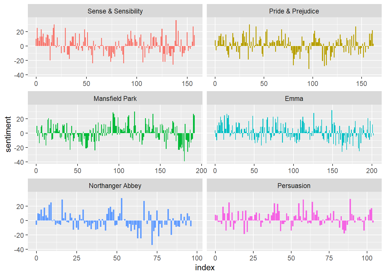
Fair to say Jane Austin novels tend to have a happy ending? The three sentiment lexicons provide different views of THE data. Here is a comparison of the lexicons using one of Jane Austin’s novels, “Pride and Prejudice”.
# AFINN lexicon measures sentiment with a numeric score between -5 and 5.
afinn <- austin_tidy %>%
  filter(book == "Pride & Prejudice") %>%
  inner_join(get_sentiments("afinn"), by = "word") %>%
  group_by(index = linenumber %/% 80) %>%
  summarise(sentiment = sum(value)) %>%
  mutate(method = "AFINN")
## `summarise()` ungrouping output (override with `.groups` argument)# Bing and nrc categorize words in a binary fashion, either positive or negative.
bing <- austin_tidy %>%
filter(book == "Pride & Prejudice") %>%
inner_join(get_sentiments("bing"), by = "word") %>%
count(index = linenumber %/% 80, sentiment) %>%
pivot_wider(names_from = sentiment, values_from = n, values_fill = list(n = 0)) %>%
mutate(sentiment = positive - negative) %>%
mutate(method = "Bing") %>%
select(index, sentiment, method)
nrc <- austin_tidy %>%
filter(book == "Pride & Prejudice") %>%
inner_join(get_sentiments("nrc") %>% filter(sentiment %in% c("positive", "negative")), by = "word") %>%
count(index = linenumber %/% 80, sentiment) %>%
pivot_wider(names_from = sentiment, values_from = n, values_fill = list(n = 0)) %>%
mutate(sentiment = positive - negative) %>%
mutate(method = "NRC") %>%
select(index, sentiment, method)
bind_rows(afinn, bing, nrc) %>%
ggplot(aes(index, sentiment, fill = method)) +
geom_col(show.legend = FALSE) +
facet_wrap(~method, ncol = 1, scales = "free_y")
In this example, and in general, NRC sentiment tends to be high, AFINN sentiment has more variance, and Bing sentiment finds longer stretches of similar text. However, all three agree roughly on the overall trends in the sentiment through a narrative arc.
What are the top-10 positive and negative words? Using the Bing lexicon, get the counts, then group_by(sentiment) and top_n() to the top 10 in each category.
austin_tidy %>%
  filter(book == "Pride & Prejudice") %>%
  inner_join(get_sentiments("bing"), by = "word") %>%
  count(word, sentiment, sort = TRUE) %>%
  group_by(sentiment) %>%
  top_n(n = 10, wt = n) %>%
  ggplot(aes(x = fct_reorder(word, n), y = n, fill = sentiment)) +
  geom_col(show.legend = FALSE) +
  facet_wrap(~sentiment, scales = "free_y") +
  coord_flip() +
  labs(y = "Contribution to Sentiment",
       x = "")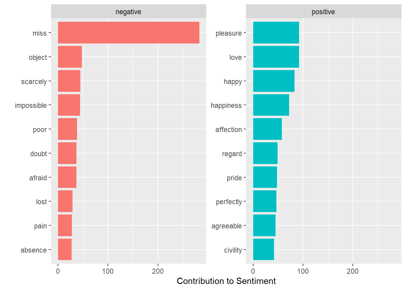
Uh oh, “miss” is a red-herring - in Jane Austin novels it often refers to an unmarried woman. Drop it from the analysis by appending it to the stop-words list.
austin_tidy %>%
  anti_join(bind_rows(stop_words,
                      tibble(word = c("miss"), lexicon = c("custom")))) %>%
  filter(book == "Pride & Prejudice") %>%
  inner_join(get_sentiments("bing")) %>%
  count(word, sentiment, sort = TRUE) %>%
  group_by(sentiment) %>%
  top_n(n = 10, wt = n) %>%
  ggplot(aes(x = fct_reorder(word, n), y = n, fill = sentiment)) +
  geom_col(show.legend = FALSE) +
  facet_wrap(~sentiment, scales = "free_y") +
  coord_flip() +
  labs(y = "Contribution to Sentiment",
       x = "")
## Joining, by = "word"
## Joining, by = "word"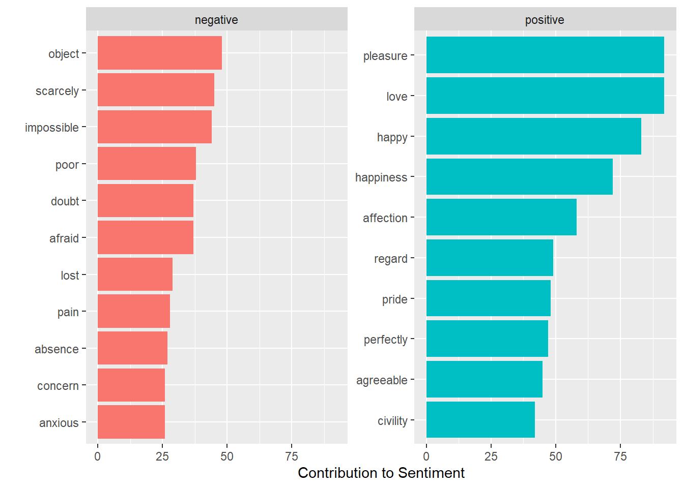
Better!
A common way to visualize sentiments is with a word cloud.
austin_tidy %>%
  anti_join(bind_rows(stop_words,
                      tibble(word = c("miss"), lexicon = c("custom")))) %>%
  filter(book == "Pride & Prejudice") %>%
  count(word) %>%
  with(wordcloud(word, n, max.words = 100))
## Joining, by = "word"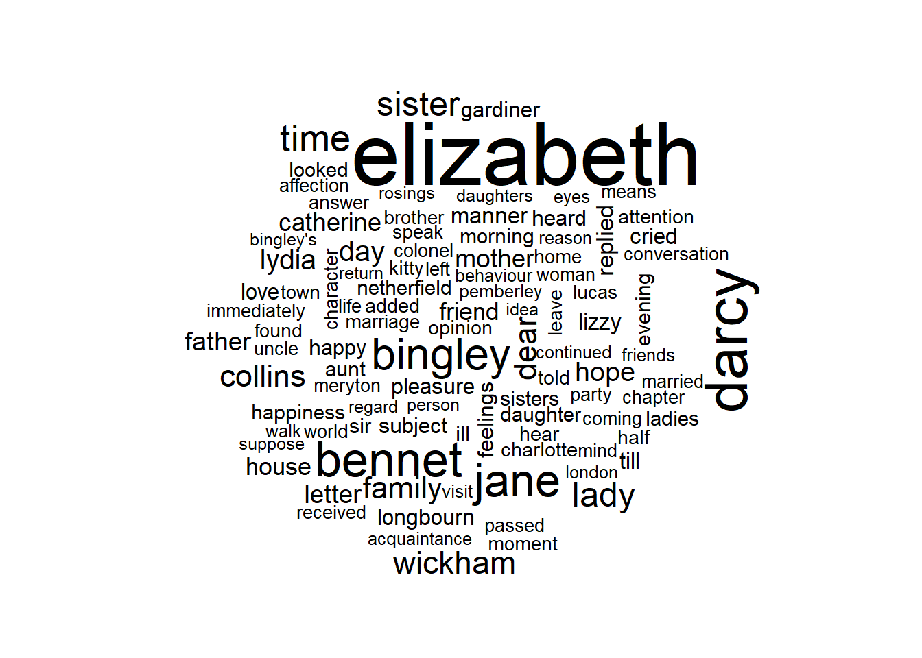
comparison.cloud is another implementation of a word cloud. It takes a matrix input.
x <- austin_tidy %>%
  anti_join(bind_rows(stop_words,
                      tibble(word = c("miss"), lexicon = c("custom")))) %>%
  inner_join(get_sentiments("bing")) %>%
  filter(book == "Pride & Prejudice") %>%
  count(word, sentiment, sort = TRUE) %>%
  pivot_wider(names_from = sentiment, values_from = n, values_fill = list(n = 0)) %>%
  as.data.frame()
## Joining, by = "word"
## Joining, by = "word"## Warning in comparison.cloud(x[, 2:3]): agreeable could not be fit on page. It
## will not be plotted.## Warning in comparison.cloud(x[, 2:3]): pleased could not be fit on page. It will
## not be plotted.## Warning in comparison.cloud(x[, 2:3]): handsome could not be fit on page. It
## will not be plotted.## Warning in comparison.cloud(x[, 2:3]): amiable could not be fit on page. It will
## not be plotted.## Warning in comparison.cloud(x[, 2:3]): advantage could not be fit on page. It
## will not be plotted.## Warning in comparison.cloud(x[, 2:3]): satisfied could not be fit on page. It
## will not be plotted.## Warning in comparison.cloud(x[, 2:3]): instantly could not be fit on page. It
## will not be plotted.## Warning in comparison.cloud(x[, 2:3]): astonishment could not be fit on page. It
## will not be plotted.## Warning in comparison.cloud(x[, 2:3]): respect could not be fit on page. It will
## not be plotted.## Warning in comparison.cloud(x[, 2:3]): compliment could not be fit on page. It
## will not be plotted.## Warning in comparison.cloud(x[, 2:3]): exceedingly could not be fit on page. It
## will not be plotted.## Warning in comparison.cloud(x[, 2:3]): admiration could not be fit on page. It
## will not be plotted.## Warning in comparison.cloud(x[, 2:3]): master could not be fit on page. It will
## not be plotted.## Warning in comparison.cloud(x[, 2:3]): pretty could not be fit on page. It will
## not be plotted.## Warning in comparison.cloud(x[, 2:3]): delighted could not be fit on page. It
## will not be plotted.## Warning in comparison.cloud(x[, 2:3]): fair could not be fit on page. It will
## not be plotted.## Warning in comparison.cloud(x[, 2:3]): favour could not be fit on page. It will
## not be plotted.## Warning in comparison.cloud(x[, 2:3]): pleasing could not be fit on page. It
## will not be plotted.## Warning in comparison.cloud(x[, 2:3]): praise could not be fit on page. It will
## not be plotted.## Warning in comparison.cloud(x[, 2:3]): proud could not be fit on page. It will
## not be plotted.## Warning in comparison.cloud(x[, 2:3]): pleasant could not be fit on page. It
## will not be plotted.## Warning in comparison.cloud(x[, 2:3]): promised could not be fit on page. It
## will not be plotted.## Warning in comparison.cloud(x[, 2:3]): charming could not be fit on page. It
## will not be plotted.## Warning in comparison.cloud(x[, 2:3]): excellent could not be fit on page. It
## will not be plotted.## Warning in comparison.cloud(x[, 2:3]): proper could not be fit on page. It will
## not be plotted.## Warning in comparison.cloud(x[, 2:3]): ready could not be fit on page. It will
## not be plotted.## Warning in comparison.cloud(x[, 2:3]): disappointment could not be fit on page.
## It will not be plotted.## Warning in comparison.cloud(x[, 2:3]): indifference could not be fit on page. It
## will not be plotted.## Warning in comparison.cloud(x[, 2:3]): resentment could not be fit on page. It
## will not be plotted.## Warning in comparison.cloud(x[, 2:3]): delightful could not be fit on page. It
## will not be plotted.## Warning in comparison.cloud(x[, 2:3]): fancy could not be fit on page. It will
## not be plotted.## Warning in comparison.cloud(x[, 2:3]): intelligence could not be fit on page. It
## will not be plotted.## Warning in comparison.cloud(x[, 2:3]): strong could not be fit on page. It will
## not be plotted.## Warning in comparison.cloud(x[, 2:3]): confess could not be fit on page. It will
## not be plotted.## Warning in comparison.cloud(x[, 2:3]): distress could not be fit on page. It
## will not be plotted.## Warning in comparison.cloud(x[, 2:3]): excuse could not be fit on page. It will
## not be plotted.## Warning in comparison.cloud(x[, 2:3]): ignorant could not be fit on page. It
## will not be plotted.## Warning in comparison.cloud(x[, 2:3]): admire could not be fit on page. It will
## not be plotted.## Warning in comparison.cloud(x[, 2:3]): capable could not be fit on page. It will
## not be plotted.## Warning in comparison.cloud(x[, 2:3]): felicity could not be fit on page. It
## will not be plotted.## Warning in comparison.cloud(x[, 2:3]): superior could not be fit on page. It
## will not be plotted.## Warning in comparison.cloud(x[, 2:3]): objection could not be fit on page. It
## will not be plotted.## Warning in comparison.cloud(x[, 2:3]): wrong could not be fit on page. It will
## not be plotted.## Warning in comparison.cloud(x[, 2:3]): affectionate could not be fit on page. It
## will not be plotted.## Warning in comparison.cloud(x[, 2:3]): ease could not be fit on page. It will
## not be plotted.## Warning in comparison.cloud(x[, 2:3]): perfect could not be fit on page. It will
## not be plotted.## Warning in comparison.cloud(x[, 2:3]): politeness could not be fit on page. It
## will not be plotted.## Warning in comparison.cloud(x[, 2:3]): promise could not be fit on page. It will
## not be plotted.## Warning in comparison.cloud(x[, 2:3]): readily could not be fit on page. It will
## not be plotted.## Warning in comparison.cloud(x[, 2:3]): disagreeable could not be fit on page. It
## will not be plotted.## Warning in comparison.cloud(x[, 2:3]): misery could not be fit on page. It will
## not be plotted.## Warning in comparison.cloud(x[, 2:3]): painful could not be fit on page. It will
## not be plotted.## Warning in comparison.cloud(x[, 2:3]): extraordinary could not be fit on page.
## It will not be plotted.## Warning in comparison.cloud(x[, 2:3]): pardon could not be fit on page. It will
## not be plotted.## Warning in comparison.cloud(x[, 2:3]): distressed could not be fit on page. It
## will not be plotted.## Warning in comparison.cloud(x[, 2:3]): interference could not be fit on page. It
## will not be plotted.## Warning in comparison.cloud(x[, 2:3]): partiality could not be fit on page. It
## will not be plotted.## Warning in comparison.cloud(x[, 2:3]): unhappy could not be fit on page. It will
## not be plotted.## Warning in comparison.cloud(x[, 2:3]): worse could not be fit on page. It will
## not be plotted.## Warning in comparison.cloud(x[, 2:3]): assurance could not be fit on page. It
## will not be plotted.## Warning in comparison.cloud(x[, 2:3]): beautiful could not be fit on page. It
## will not be plotted.## Warning in comparison.cloud(x[, 2:3]): earnest could not be fit on page. It will
## not be plotted.## Warning in comparison.cloud(x[, 2:3]): worth could not be fit on page. It will
## not be plotted.## Warning in comparison.cloud(x[, 2:3]): apprehension could not be fit on page. It
## will not be plotted.## Warning in comparison.cloud(x[, 2:3]): contempt could not be fit on page. It
## will not be plotted.## Warning in comparison.cloud(x[, 2:3]): disappointed could not be fit on page. It
## will not be plotted.## Warning in comparison.cloud(x[, 2:3]): astonished could not be fit on page. It
## will not be plotted.## Warning in comparison.cloud(x[, 2:3]): compassion could not be fit on page. It
## will not be plotted.## Warning in comparison.cloud(x[, 2:3]): eagerly could not be fit on page. It will
## not be plotted.## Warning in comparison.cloud(x[, 2:3]): elegant could not be fit on page. It will
## not be plotted.## Warning in comparison.cloud(x[, 2:3]): gratified could not be fit on page. It
## will not be plotted.## Warning in comparison.cloud(x[, 2:3]): reasonable could not be fit on page. It
## will not be plotted.## Warning in comparison.cloud(x[, 2:3]): respectable could not be fit on page. It
## will not be plotted.## Warning in comparison.cloud(x[, 2:3]): tolerable could not be fit on page. It
## will not be plotted.## Warning in comparison.cloud(x[, 2:3]): eager could not be fit on page. It will
## not be plotted.## Warning in comparison.cloud(x[, 2:3]): enjoyment could not be fit on page. It
## will not be plotted.## Warning in comparison.cloud(x[, 2:3]): grateful could not be fit on page. It
## will not be plotted.## Warning in comparison.cloud(x[, 2:3]): intimate could not be fit on page. It
## will not be plotted.## Warning in comparison.cloud(x[, 2:3]): relief could not be fit on page. It will
## not be plotted.## Warning in comparison.cloud(x[, 2:3]): secure could not be fit on page. It will
## not be plotted.## Warning in comparison.cloud(x[, 2:3]): confusion could not be fit on page. It
## will not be plotted.## Warning in comparison.cloud(x[, 2:3]): difficult could not be fit on page. It
## will not be plotted.## Warning in comparison.cloud(x[, 2:3]): disgrace could not be fit on page. It
## will not be plotted.## Warning in comparison.cloud(x[, 2:3]): dreadful could not be fit on page. It
## will not be plotted.## Warning in comparison.cloud(x[, 2:3]): excessively could not be fit on page. It
## will not be plotted.## Warning in comparison.cloud(x[, 2:3]): imprudent could not be fit on page. It
## will not be plotted.## Warning in comparison.cloud(x[, 2:3]): neglect could not be fit on page. It will
## not be plotted.## Warning in comparison.cloud(x[, 2:3]): objections could not be fit on page. It
## will not be plotted.## Warning in comparison.cloud(x[, 2:3]): accomplished could not be fit on page. It
## will not be plotted.## Warning in comparison.cloud(x[, 2:3]): comfortable could not be fit on page. It
## will not be plotted.## Warning in comparison.cloud(x[, 2:3]): congratulations could not be fit on page.
## It will not be plotted.## Warning in comparison.cloud(x[, 2:3]): courage could not be fit on page. It will
## not be plotted.## Warning in comparison.cloud(x[, 2:3]): generous could not be fit on page. It
## will not be plotted.## Warning in comparison.cloud(x[, 2:3]): recommend could not be fit on page. It
## will not be plotted.## Warning in comparison.cloud(x[, 2:3]): steady could not be fit on page. It will
## not be plotted.## Warning in comparison.cloud(x[, 2:3]): awkward could not be fit on page. It will
## not be plotted.## Warning in comparison.cloud(x[, 2:3]): debts could not be fit on page. It will
## not be plotted.## Warning in comparison.cloud(x[, 2:3]): embarrassment could not be fit on page.
## It will not be plotted.## Warning in comparison.cloud(x[, 2:3]): impatience could not be fit on page. It
## will not be plotted.## Warning in comparison.cloud(x[, 2:3]): insufficient could not be fit on page. It
## will not be plotted.## Warning in comparison.cloud(x[, 2:3]): interruption could not be fit on page. It
## will not be plotted.## Warning in comparison.cloud(x[, 2:3]): shame could not be fit on page. It will
## not be plotted.## Warning in comparison.cloud(x[, 2:3]): strange could not be fit on page. It will
## not be plotted.## Warning in comparison.cloud(x[, 2:3]): unlucky could not be fit on page. It will
## not be plotted.## Warning in comparison.cloud(x[, 2:3]): unwilling could not be fit on page. It
## will not be plotted.## Warning in comparison.cloud(x[, 2:3]): vexation could not be fit on page. It
## will not be plotted.## Warning in comparison.cloud(x[, 2:3]): wretched could not be fit on page. It
## will not be plotted.## Warning in comparison.cloud(x[, 2:3]): confidence could not be fit on page. It
## will not be plotted.## Warning in comparison.cloud(x[, 2:3]): delicacy could not be fit on page. It
## will not be plotted.## Warning in comparison.cloud(x[, 2:3]): earnestly could not be fit on page. It
## will not be plotted.## Warning in comparison.cloud(x[, 2:3]): gained could not be fit on page. It will
## not be plotted.## Warning in comparison.cloud(x[, 2:3]): noble could not be fit on page. It will
## not be plotted.## Warning in comparison.cloud(x[, 2:3]): satisfy could not be fit on page. It will
## not be plotted.## Warning in comparison.cloud(x[, 2:3]): fears could not be fit on page. It will
## not be plotted.## Warning in comparison.cloud(x[, 2:3]): haste could not be fit on page. It will
## not be plotted.## Warning in comparison.cloud(x[, 2:3]): hastily could not be fit on page. It will
## not be plotted.## Warning in comparison.cloud(x[, 2:3]): imprudence could not be fit on page. It
## will not be plotted.## Warning in comparison.cloud(x[, 2:3]): misfortune could not be fit on page. It
## will not be plotted.## Warning in comparison.cloud(x[, 2:3]): mistress could not be fit on page. It
## will not be plotted.## Warning in comparison.cloud(x[, 2:3]): refuse could not be fit on page. It will
## not be plotted.## Warning in comparison.cloud(x[, 2:3]): suspicion could not be fit on page. It
## will not be plotted.## Warning in comparison.cloud(x[, 2:3]): violent could not be fit on page. It will
## not be plotted.## Warning in comparison.cloud(x[, 2:3]): attentive could not be fit on page. It
## will not be plotted.## Warning in comparison.cloud(x[, 2:3]): encouragement could not be fit on page.
## It will not be plotted.## Warning in comparison.cloud(x[, 2:3]): excited could not be fit on page. It will
## not be plotted.## Warning in comparison.cloud(x[, 2:3]): flatter could not be fit on page. It will
## not be plotted.## Warning in comparison.cloud(x[, 2:3]): goodness could not be fit on page. It
## will not be plotted.## Warning in comparison.cloud(x[, 2:3]): heartily could not be fit on page. It
## will not be plotted.## Warning in comparison.cloud(x[, 2:3]): heaven could not be fit on page. It will
## not be plotted.## Warning in comparison.cloud(x[, 2:3]): intimacy could not be fit on page. It
## will not be plotted.## Warning in comparison.cloud(x[, 2:3]): rational could not be fit on page. It
## will not be plotted.## Warning in comparison.cloud(x[, 2:3]): remarkably could not be fit on page. It
## will not be plotted.## Warning in comparison.cloud(x[, 2:3]): sincere could not be fit on page. It will
## not be plotted.## Warning in comparison.cloud(x[, 2:3]): smiles could not be fit on page. It will
## not be plotted.## Warning in comparison.cloud(x[, 2:3]): smiling could not be fit on page. It will
## not be plotted.## Warning in comparison.cloud(x[, 2:3]): triumph could not be fit on page. It will
## not be plotted.## Warning in comparison.cloud(x[, 2:3]): virtue could not be fit on page. It will
## not be plotted.## Warning in comparison.cloud(x[, 2:3]): alarmed could not be fit on page. It will
## not be plotted.## Warning in comparison.cloud(x[, 2:3]): concerns could not be fit on page. It
## will not be plotted.## Warning in comparison.cloud(x[, 2:3]): death could not be fit on page. It will
## not be plotted.## Warning in comparison.cloud(x[, 2:3]): deny could not be fit on page. It will
## not be plotted.## Warning in comparison.cloud(x[, 2:3]): difficulty could not be fit on page. It
## will not be plotted.## Warning in comparison.cloud(x[, 2:3]): evils could not be fit on page. It will
## not be plotted.## Warning in comparison.cloud(x[, 2:3]): foolish could not be fit on page. It will
## not be plotted.## Warning in comparison.cloud(x[, 2:3]): impatient could not be fit on page. It
## will not be plotted.## Warning in comparison.cloud(x[, 2:3]): incapable could not be fit on page. It
## will not be plotted.## Warning in comparison.cloud(x[, 2:3]): indignation could not be fit on page. It
## will not be plotted.## Warning in comparison.cloud(x[, 2:3]): mistake could not be fit on page. It will
## not be plotted.## Warning in comparison.cloud(x[, 2:3]): nonsense could not be fit on page. It
## will not be plotted.## Warning in comparison.cloud(x[, 2:3]): protested could not be fit on page. It
## will not be plotted.## Warning in comparison.cloud(x[, 2:3]): reproach could not be fit on page. It
## will not be plotted.## Warning in comparison.cloud(x[, 2:3]): severe could not be fit on page. It will
## not be plotted.## Warning in comparison.cloud(x[, 2:3]): shocked could not be fit on page. It will
## not be plotted.## Warning in comparison.cloud(x[, 2:3]): solicitude could not be fit on page. It
## will not be plotted.## Warning in comparison.cloud(x[, 2:3]): suffered could not be fit on page. It
## will not be plotted.## Warning in comparison.cloud(x[, 2:3]): uneasy could not be fit on page. It will
## not be plotted.## Warning in comparison.cloud(x[, 2:3]): unexpected could not be fit on page. It
## will not be plotted.## Warning in comparison.cloud(x[, 2:3]): unknown could not be fit on page. It will
## not be plotted.## Warning in comparison.cloud(x[, 2:3]): unpleasant could not be fit on page. It
## will not be plotted.## Warning in comparison.cloud(x[, 2:3]): elegance could not be fit on page. It
## will not be plotted.## Warning in comparison.cloud(x[, 2:3]): fresh could not be fit on page. It will
## not be plotted.## Warning in comparison.cloud(x[, 2:3]): humble could not be fit on page. It will
## not be plotted.## Warning in comparison.cloud(x[, 2:3]): improvement could not be fit on page. It
## will not be plotted.## Warning in comparison.cloud(x[, 2:3]): patience could not be fit on page. It
## will not be plotted.## Warning in comparison.cloud(x[, 2:3]): recommended could not be fit on page. It
## will not be plotted.## Warning in comparison.cloud(x[, 2:3]): sincerely could not be fit on page. It
## will not be plotted.## Warning in comparison.cloud(x[, 2:3]): valuable could not be fit on page. It
## will not be plotted.## Warning in comparison.cloud(x[, 2:3]): broken could not be fit on page. It will
## not be plotted.## Warning in comparison.cloud(x[, 2:3]): condescension could not be fit on page.
## It will not be plotted.## Warning in comparison.cloud(x[, 2:3]): disapprobation could not be fit on page.
## It will not be plotted.## Warning in comparison.cloud(x[, 2:3]): falsehood could not be fit on page. It
## will not be plotted.## Warning in comparison.cloud(x[, 2:3]): fault could not be fit on page. It will
## not be plotted.## Warning in comparison.cloud(x[, 2:3]): hopeless could not be fit on page. It
## will not be plotted.## Warning in comparison.cloud(x[, 2:3]): ignorance could not be fit on page. It
## will not be plotted.## Warning in comparison.cloud(x[, 2:3]): improbable could not be fit on page. It
## will not be plotted.## Warning in comparison.cloud(x[, 2:3]): refusal could not be fit on page. It will
## not be plotted.## Warning in comparison.cloud(x[, 2:3]): refusing could not be fit on page. It
## will not be plotted.## Warning in comparison.cloud(x[, 2:3]): selfish could not be fit on page. It will
## not be plotted.## Warning in comparison.cloud(x[, 2:3]): temptation could not be fit on page. It
## will not be plotted.## Warning in comparison.cloud(x[, 2:3]): uncomfortable could not be fit on page.
## It will not be plotted.## Warning in comparison.cloud(x[, 2:3]): uneasiness could not be fit on page. It
## will not be plotted.## Warning in comparison.cloud(x[, 2:3]): unreasonable could not be fit on page. It
## will not be plotted.## Warning in comparison.cloud(x[, 2:3]): weak could not be fit on page. It will
## not be plotted.## Warning in comparison.cloud(x[, 2:3]): worst could not be fit on page. It will
## not be plotted.## Warning in comparison.cloud(x[, 2:3]): assurances could not be fit on page. It
## will not be plotted.## Warning in comparison.cloud(x[, 2:3]): eagerness could not be fit on page. It
## will not be plotted.## Warning in comparison.cloud(x[, 2:3]): enjoy could not be fit on page. It will
## not be plotted.## Warning in comparison.cloud(x[, 2:3]): gracious could not be fit on page. It
## will not be plotted.## Warning in comparison.cloud(x[, 2:3]): indebted could not be fit on page. It
## will not be plotted.## Warning in comparison.cloud(x[, 2:3]): openly could not be fit on page. It will
## not be plotted.## Warning in comparison.cloud(x[, 2:3]): properly could not be fit on page. It
## will not be plotted.## Warning in comparison.cloud(x[, 2:3]): quiet could not be fit on page. It will
## not be plotted.## Warning in comparison.cloud(x[, 2:3]): thankful could not be fit on page. It
## will not be plotted.## Warning in comparison.cloud(x[, 2:3]): warmly could not be fit on page. It will
## not be plotted.## Warning in comparison.cloud(x[, 2:3]): warmth could not be fit on page. It will
## not be plotted.## Warning in comparison.cloud(x[, 2:3]): abominable could not be fit on page. It
## will not be plotted.## Warning in comparison.cloud(x[, 2:3]): delayed could not be fit on page. It will
## not be plotted.## Warning in comparison.cloud(x[, 2:3]): disdain could not be fit on page. It will
## not be plotted.## Warning in comparison.cloud(x[, 2:3]): displeasure could not be fit on page. It
## will not be plotted.## Warning in comparison.cloud(x[, 2:3]): distressing could not be fit on page. It
## will not be plotted.## Warning in comparison.cloud(x[, 2:3]): hurt could not be fit on page. It will
## not be plotted.## Warning in comparison.cloud(x[, 2:3]): impertinent could not be fit on page. It
## will not be plotted.## Warning in comparison.cloud(x[, 2:3]): inconvenience could not be fit on page.
## It will not be plotted.## Warning in comparison.cloud(x[, 2:3]): miserable could not be fit on page. It
## will not be plotted.## Warning in comparison.cloud(x[, 2:3]): mortification could not be fit on page.
## It will not be plotted.## Warning in comparison.cloud(x[, 2:3]): mortifying could not be fit on page. It
## will not be plotted.## Warning in comparison.cloud(x[, 2:3]): prejudice could not be fit on page. It
## will not be plotted.## Warning in comparison.cloud(x[, 2:3]): refused could not be fit on page. It will
## not be plotted.## Warning in comparison.cloud(x[, 2:3]): resigned could not be fit on page. It
## will not be plotted.## Warning in comparison.cloud(x[, 2:3]): sick could not be fit on page. It will
## not be plotted.## Warning in comparison.cloud(x[, 2:3]): useless could not be fit on page. It will
## not be plotted.## Warning in comparison.cloud(x[, 2:3]): violently could not be fit on page. It
## will not be plotted.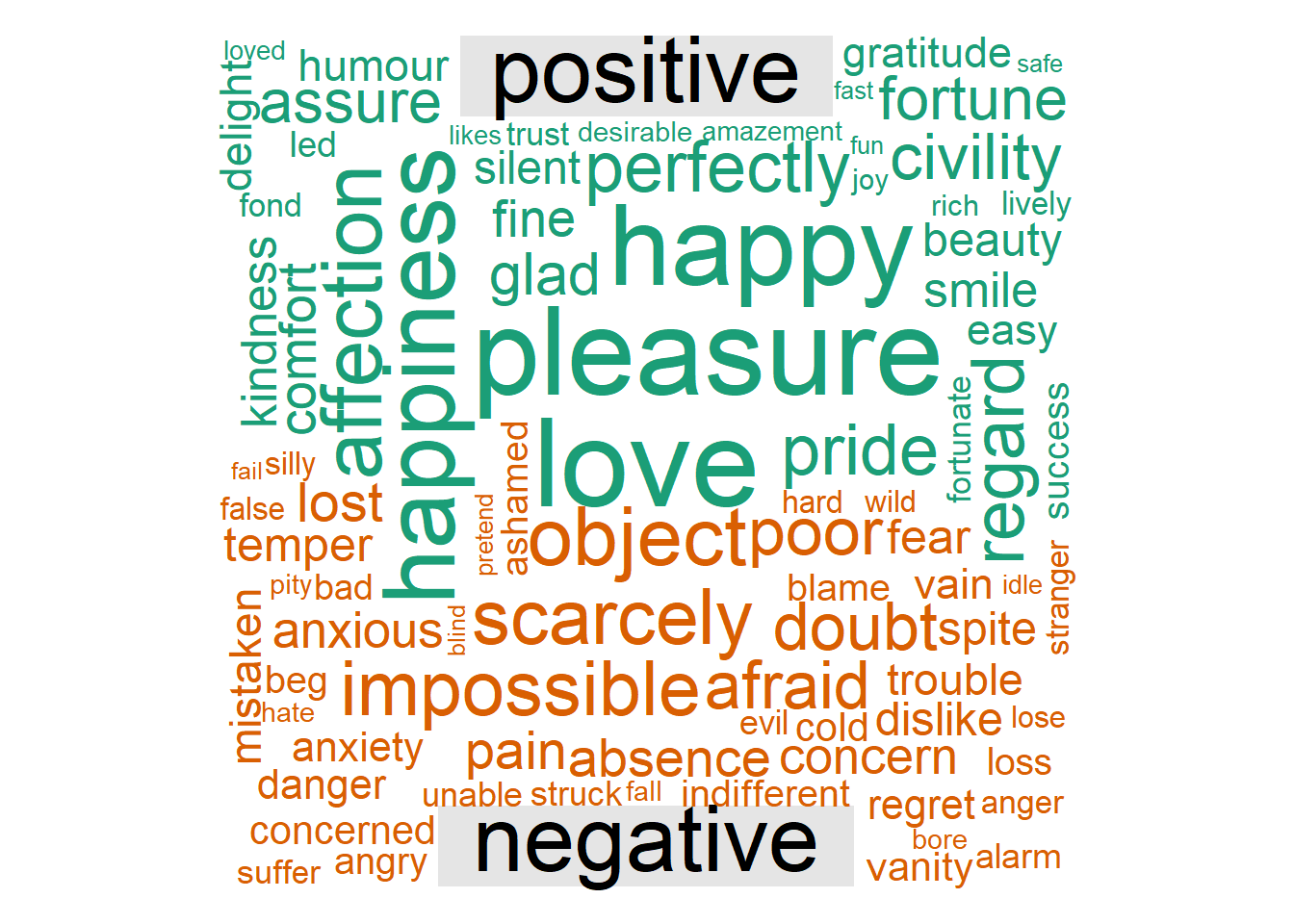
Sometimes it makes more sense to analyze entire sentences. Specify unnest_tokens(..., token = "sentences") to override the default token = "word".
austen_books() %>%
group_by(book) %>%
mutate(linenumber = row_number(),
chapter = cumsum(str_detect(text, regex("^chapter [\\divxlc]",
ignore_case = TRUE)))) %>%
ungroup() %>%
unnest_tokens(output = word, input = text, token = "sentences")## # A tibble: 87,906 x 4
## book linenumber chapter word
## <fct> <int> <int> <chr>
## 1 Sense & Sensi~ 1 0 sense and sensibility
## 2 Sense & Sensi~ 3 0 by jane austen
## 3 Sense & Sensi~ 5 0 (1811)
## 4 Sense & Sensi~ 10 1 chapter 1
## 5 Sense & Sensi~ 13 1 the family of dashwood had long been settl~
## 6 Sense & Sensi~ 13 1 their estate
## 7 Sense & Sensi~ 14 1 was large, and their residence was at norl~
## 8 Sense & Sensi~ 15 1 their property, where, for many generation~
## 9 Sense & Sensi~ 16 1 respectable a manner as to engage the gene~
## 10 Sense & Sensi~ 17 1 surrounding acquaintance.
## # ... with 87,896 more rows13.3.1 N-Grams
Create n-grams by specifying unnest_tokens(..., token = "ngrams", n) where n = 2 is a bigram, etc. To remove the stop words, separate the n-grams, then filter on the stop_words data set.
austin.2gram <- austen_books() %>%
group_by(book) %>%
mutate(linenumber = row_number(),
chapter = cumsum(str_detect(text, regex("^chapter [\\divxlc]",
ignore_case = TRUE)))) %>%
ungroup() %>%
unnest_tokens(output = bigram, input = text, token = "ngrams", n = 2)
austin.2gram <- austin.2gram %>%
separate(bigram, c("word1", "word2"), sep = " ") %>%
filter(!word1 %in% stop_words$word &
!word2 %in% stop_words$word &
!is.na(word1) & !is.na(word2)) %>%
unite(bigram, word1, word2, sep = " ")
austin.2gram %>%
count(book, bigram, sort = TRUE)## # A tibble: 31,391 x 3
## book bigram n
## <fct> <chr> <int>
## 1 Mansfield Park sir thomas 266
## 2 Mansfield Park miss crawford 196
## 3 Emma miss woodhouse 143
## 4 Persuasion captain wentworth 143
## 5 Emma frank churchill 114
## 6 Persuasion lady russell 110
## 7 Persuasion sir walter 108
## 8 Mansfield Park lady bertram 101
## 9 Emma miss fairfax 98
## 10 Sense & Sensibility colonel brandon 96
## # ... with 31,381 more rowsHere are the most commonly mentioned streets in Austin’s novels.
austin.2gram %>%
separate(bigram, c("word1", "word2"), sep = " ") %>%
filter(word2 == "street") %>%
count(book, word1, sort = TRUE)## # A tibble: 33 x 3
## book word1 n
## <fct> <chr> <int>
## 1 Sense & Sensibility harley 16
## 2 Sense & Sensibility berkeley 15
## 3 Northanger Abbey milsom 10
## 4 Northanger Abbey pulteney 10
## 5 Mansfield Park wimpole 9
## 6 Pride & Prejudice gracechurch 8
## 7 Persuasion milsom 5
## 8 Sense & Sensibility bond 4
## 9 Sense & Sensibility conduit 4
## 10 Persuasion rivers 4
## # ... with 23 more rowsBind the tf-idf statistics. Tf-idf is short for term frequency–inverse document frequency. It is a statistic that indicates how important a word is to a document in a collection or corpus. Tf–idf increases with the number of times a word appears in the document and decreases with the number of documents in the corpus that contain the word. The idf adjusts for the fact that some words appear more frequently in general.
austen_books() %>%
group_by(book) %>%
mutate(linenumber = row_number(),
chapter = cumsum(str_detect(text, regex("^chapter [\\divxlc]",
ignore_case = TRUE)))) %>%
ungroup() %>%
unnest_tokens(output = bigram, input = text, token = "ngrams", n = 2) %>%
separate(bigram, c("word1", "word2"), sep = " ") %>%
filter(!word1 %in% stop_words$word &
!word2 %in% stop_words$word &
!is.na(word1) & !is.na(word2)) %>%
unite(bigram, word1, word2, sep = " ")## # A tibble: 38,913 x 4
## book linenumber chapter bigram
## <fct> <int> <int> <chr>
## 1 Sense & Sensibility 3 0 jane austen
## 2 Sense & Sensibility 10 1 chapter 1
## 3 Sense & Sensibility 14 1 norland park
## 4 Sense & Sensibility 17 1 surrounding acquaintance
## 5 Sense & Sensibility 17 1 late owner
## 6 Sense & Sensibility 18 1 advanced age
## 7 Sense & Sensibility 19 1 constant companion
## 8 Sense & Sensibility 20 1 happened ten
## 9 Sense & Sensibility 22 1 henry dashwood
## 10 Sense & Sensibility 23 1 norland estate
## # ... with 38,903 more rowsaustin.2gram %>%
count(book, bigram) %>%
bind_tf_idf(bigram, book, n) %>%
group_by(book) %>%
top_n(n = 10, wt = tf_idf) %>%
ggplot(aes(x = fct_reorder(bigram, n), y = tf_idf, fill = book)) +
geom_col(show.legend = FALSE) +
facet_wrap(~book, scales = "free_y", ncol = 2) +
labs(y = "tf-idf of bigram to novel") +
coord_flip() 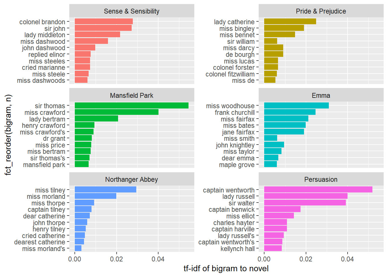
A good way to visualize bigrams is with a network graph. Packages igraph and ggraph provides tools for this purpose.
set.seed(2016)
austen_books() %>%
group_by(book) %>%
mutate(linenumber = row_number(),
chapter = cumsum(str_detect(text, regex("^chapter [\\divxlc]",
ignore_case = TRUE)))) %>%
ungroup() %>%
unnest_tokens(output = bigram, input = text, token = "ngrams", n = 2) %>%
separate(bigram, c("word1", "word2"), sep = " ") %>%
filter(!word1 %in% stop_words$word &
!word2 %in% stop_words$word &
!is.na(word1) & !is.na(word2)) %>%
count(word1, word2) %>%
filter(n > 20) %>%
graph_from_data_frame() %>% # creates unformatted "graph"
ggraph(layout = "fr") +
geom_edge_link(aes(edge_alpha = n),
show.legend = FALSE,
arrow = grid::arrow(type = "closed",
length = unit(.15, "inches")),
end_cap = circle(.07, 'inches')) +
geom_node_point(color = "lightblue",
size = 5) +
geom_node_text(aes(label = name), vjust = 1, hjust = 1) +
theme_void()
If you want to count the number of times that two words appear within the same document, or to see how correlated they are, widen the data with the widyr package.
austen_books() %>%
filter(book == "Pride & Prejudice") %>%
mutate(section = row_number() %/% 10) %>%
filter(section > 0) %>%
unnest_tokens(word, text) %>%
filter(!word %in% stop_words$word) %>%
pairwise_count(word, section, sort = TRUE)## Warning: `distinct_()` is deprecated as of dplyr 0.7.0.
## Please use `distinct()` instead.
## See vignette('programming') for more help
## This warning is displayed once every 8 hours.
## Call `lifecycle::last_warnings()` to see where this warning was generated.## Warning: `tbl_df()` is deprecated as of dplyr 1.0.0.
## Please use `tibble::as_tibble()` instead.
## This warning is displayed once every 8 hours.
## Call `lifecycle::last_warnings()` to see where this warning was generated.## # A tibble: 796,008 x 3
## item1 item2 n
## <chr> <chr> <dbl>
## 1 darcy elizabeth 144
## 2 elizabeth darcy 144
## 3 miss elizabeth 110
## 4 elizabeth miss 110
## 5 elizabeth jane 106
## 6 jane elizabeth 106
## 7 miss darcy 92
## 8 darcy miss 92
## 9 elizabeth bingley 91
## 10 bingley elizabeth 91
## # ... with 795,998 more rowsThe correlation among words is how often they appear together relative to how often they appear separately. The phi coefficient is defined
\[\phi = \frac{n_{11}n_{00} - n_{10}n_{01}}{\sqrt{n_{1.}n_{0.}n_{.1}n_{.0}}}\]
where \(n_{10}\) means number of times section has word x, but not word y, and \(n_{1.}\) means total times section has word x. This lets us pick particular interesting words and find the other words most associated with them.
austen_books() %>%
filter(book == "Pride & Prejudice") %>%
mutate(section = row_number() %/% 10) %>%
filter(section > 0) %>%
unnest_tokens(word, text) %>%
filter(!word %in% stop_words$word) %>%
pairwise_cor(word, section, sort = TRUE) %>%
filter(item1 %in% c("elizabeth", "pounds", "married", "pride")) %>%
group_by(item1) %>%
top_n(n = 4) %>%
ungroup() %>%
mutate(item2 = reorder(item2, correlation)) %>%
ggplot(aes(x = item2, y = correlation)) +
geom_bar(stat = "identity") +
facet_wrap(~ item1, scales = "free") +
coord_flip()## Selecting by correlation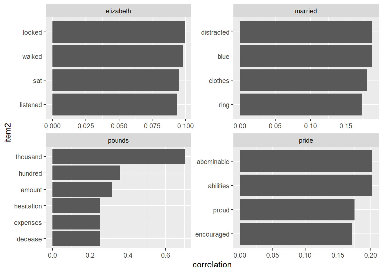
You can use the correlation to set a threshold for a graph.
set.seed(2016)
austen_books() %>%
filter(book == "Pride & Prejudice") %>%
mutate(section = row_number() %/% 10) %>%
filter(section > 0) %>%
unnest_tokens(word, text) %>%
filter(!word %in% stop_words$word) %>%
# filter to relatively common words
group_by(word) %>%
filter(n() > 20) %>%
pairwise_cor(word, section, sort = TRUE) %>%
filter(correlation > .15) %>% # relatively correlated words
graph_from_data_frame() %>%
ggraph(layout = "fr") +
geom_edge_link(aes(edge_alpha = correlation), show.legend = FALSE) +
geom_node_point(color = "lightblue", size = 5) +
geom_node_text(aes(label = name), repel = TRUE) +
theme_void()
13.3.2 Converting to and from non-tidy formats
One of the most common objects in text mining packages is the document term matrix (DTM) where each row is a document, each column a term, and each value an appearance count. The broom package contains functions to convert between DTM and tidy formats.
Convert a DTM object into a tidy data frame with tidy(). Convert a tidy object into a sparse matrix with cast_sparse(), into a DTM with cast_dtm(), and into a “dfm” for quanteda with cast_dfm().
## <<DocumentTermMatrix (documents: 2246, terms: 10473)>>
## Non-/sparse entries: 302031/23220327
## Sparsity : 99%
## Maximal term length: 18
## Weighting : term frequency (tf)## [1] "aaron" "abandon" "abandoned" "abandoning" "abbott"
## [6] "abboud"Create a tidy version of AssociatedPress with tidy().
ap_td <- tidy(AssociatedPress)
ap_td %>%
inner_join(get_sentiments("bing"), by = c(term = "word")) %>%
count(sentiment, term, wt = count) %>%
ungroup() %>%
filter(n >= 200) %>%
mutate(n = ifelse(sentiment == "negative", -n, n)) %>%
arrange(n) %>%
ggplot(aes(x = fct_inorder(term), y = n, fill = sentiment)) +
geom_bar(stat = "identity") +
labs(title = "Most Common AP Sentiment Words",
x = "",
y = "Contribution to Sentiment") +
theme(legend.position = "top",
legend.title = element_blank()) +
coord_flip()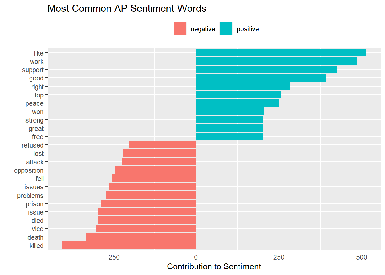
The document-feature matrix dfm class from the quanteda text-mining package is another implementation of a document-term matrix. Here are the terms most specific (highest tf-idf) from each of four selected inaugural addresses.
data("data_corpus_inaugural", package = "quanteda")
inaug_dfm <- quanteda::dfm(data_corpus_inaugural, verbose = FALSE)
head(inaug_dfm)## Document-feature matrix of: 6 documents, 9,360 features (93.8% sparse) and 4 docvars.
## features
## docs fellow-citizens of the senate and house representatives :
## 1789-Washington 1 71 116 1 48 2 2 1
## 1793-Washington 0 11 13 0 2 0 0 1
## 1797-Adams 3 140 163 1 130 0 2 0
## 1801-Jefferson 2 104 130 0 81 0 0 1
## 1805-Jefferson 0 101 143 0 93 0 0 0
## 1809-Madison 1 69 104 0 43 0 0 0
## features
## docs among vicissitudes
## 1789-Washington 1 1
## 1793-Washington 0 0
## 1797-Adams 4 0
## 1801-Jefferson 1 0
## 1805-Jefferson 7 0
## 1809-Madison 0 0
## [ reached max_nfeat ... 9,350 more features ]## # A tibble: 6 x 3
## document term count
## <chr> <chr> <dbl>
## 1 1789-Washington fellow-citizens 1
## 2 1797-Adams fellow-citizens 3
## 3 1801-Jefferson fellow-citizens 2
## 4 1809-Madison fellow-citizens 1
## 5 1813-Madison fellow-citizens 1
## 6 1817-Monroe fellow-citizens 5inaug_td %>%
bind_tf_idf(term = term, document = document, n = count) %>%
group_by(document) %>%
top_n(n = 10, wt = tf_idf) %>%
ungroup() %>%
filter(document %in% c("1861-Lincoln", "1933-Roosevelt", "1961-Kennedy", "2009-Obama")) %>%
arrange(document, desc(tf_idf)) %>%
ggplot(aes(x = fct_rev(fct_inorder(term)), y = tf_idf, fill = document)) +
geom_col() +
labs(x = "") +
theme(legend.position = "none") +
coord_flip() +
facet_wrap(~document, ncol = 2, scales = "free")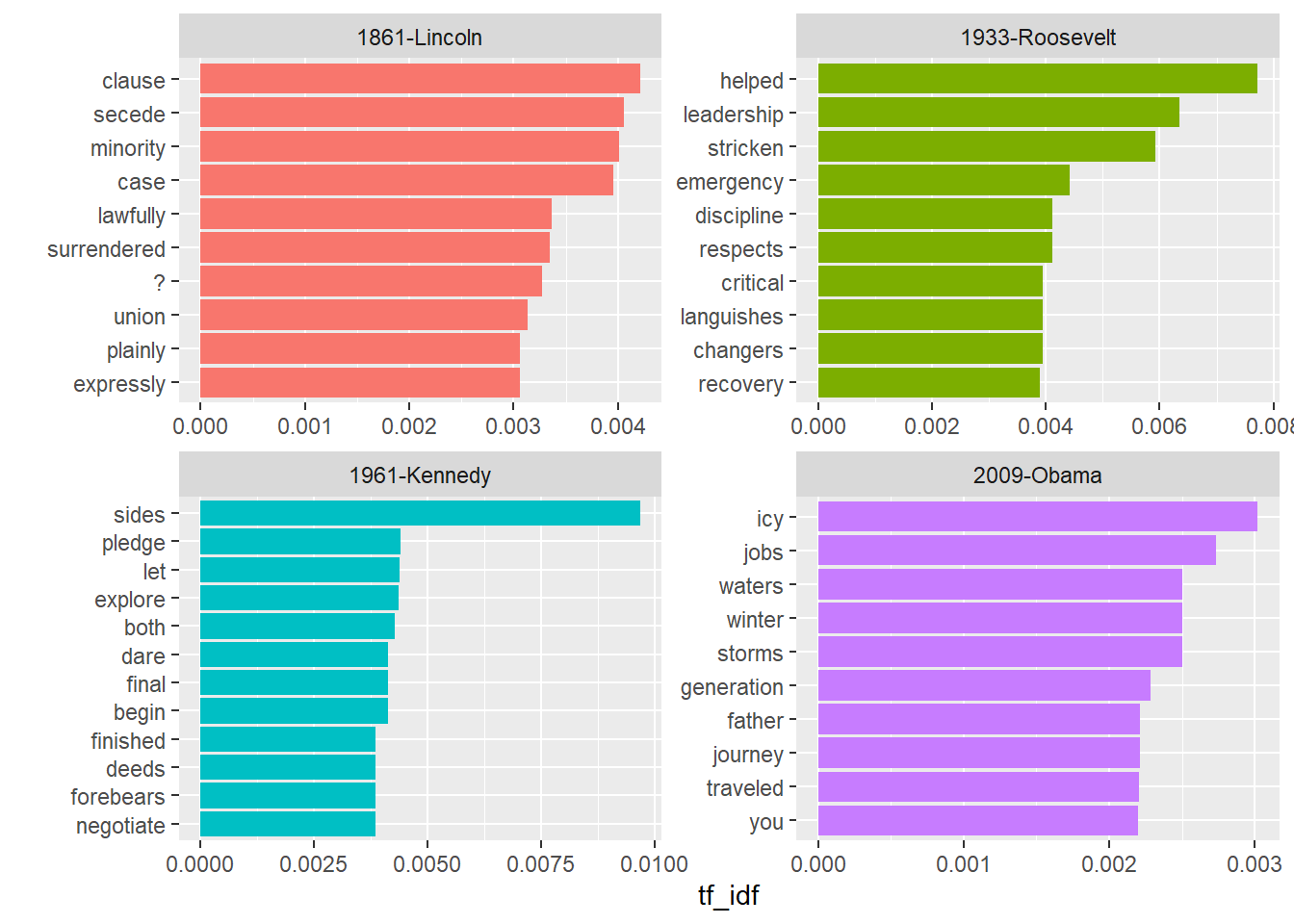
And here is word frequency trend ocer time for six selected terms. (problem with extract() below).
# inaug_td %>%
# extract(document, "year", "(\\d+)", convert = TRUE) %>%
# complete(year, term, fill = list(count = 0)) %>%
# group_by(year) %>%
# mutate(year_total = sum(count)) %>%
# filter(term %in% c("god", "america", "foreign", "union", "constitution", "freedom")) %>%
# ggplot(aes(x = year, y = count / year_total)) +
# geom_point() +
# geom_smooth() +
# facet_wrap(~ term, scales = "free_y") +
# scale_y_continuous(labels = scales::percent_format()) +
# labs(y = "",
# title = "% frequency of word in inaugural address")Cast tidy data into document-term matrix with cast_dtm(), quanteda’s dfm with cast_dfm(), and sparese matrix with cast_sparse().
inaug_dtm <- cast_dtm(data = inaug_td, document = document, term = term, value = count)
inaug_dfm <- cast_dfm(data = inaug_td, document = document, term = term, value = count)
inaug_sparse <- cast_sparse(data = inaug_td, row = document, column = term, value = count)An untokenized document collection is called a corpus. The corpuse may include metadata, such as ID, date/time, title, language, etc. Corpus metadata is usually stored as lists. Use tidy() to construct a table, one row per document.
## <<VCorpus>>
## Metadata: corpus specific: 0, document level (indexed): 0
## Content: documents: 50## <<PlainTextDocument>>
## Metadata: 15
## Content: chars: 1287## # A tibble: 50 x 16
## author datetimestamp description heading id language origin topics
## <chr> <dttm> <chr> <chr> <chr> <chr> <chr> <chr>
## 1 <NA> 1987-02-26 10:18:06 "" COMPUT~ 10 en Reute~ YES
## 2 <NA> 1987-02-26 10:19:15 "" OHIO M~ 12 en Reute~ YES
## 3 <NA> 1987-02-26 10:49:56 "" MCLEAN~ 44 en Reute~ YES
## 4 By Ca~ 1987-02-26 10:51:17 "" CHEMLA~ 45 en Reute~ YES
## 5 <NA> 1987-02-26 11:08:33 "" <COFAB~ 68 en Reute~ YES
## 6 <NA> 1987-02-26 11:32:37 "" INVEST~ 96 en Reute~ YES
## 7 By Pa~ 1987-02-26 11:43:13 "" AMERIC~ 110 en Reute~ YES
## 8 <NA> 1987-02-26 11:59:25 "" HONG K~ 125 en Reute~ YES
## 9 <NA> 1987-02-26 12:01:28 "" LIEBER~ 128 en Reute~ YES
## 10 <NA> 1987-02-26 12:08:27 "" GULF A~ 134 en Reute~ YES
## # ... with 40 more rows, and 8 more variables: lewissplit <chr>,
## # cgisplit <chr>, oldid <chr>, places <named list>, people <lgl>, orgs <lgl>,
## # exchanges <lgl>, text <chr>13.3.3 Example
Library tm.plugin.webmining connects to online feeds to retrieve news articles based on a keyword.
## Warning: package 'tm.plugin.webmining' was built under R version 4.0.2##
## Attaching package: 'tm.plugin.webmining'## The following object is masked from 'package:tidyr':
##
## extract## The following object is masked from 'package:base':
##
## parselibrary(purrr)
company <- c("Progressive", "Microsoft", "Apple")
symbol <- c("PRG", "MSFT", "AAPL")
download_articles <- function(symbol) {
WebCorpus(GoogleFinanceSource(paste0("NASDAQ:", symbol)))
}
#stock_articles <- tibble(company = company,
# symbol = symbol) %>%
# mutate(corpus = map(symbol, download_articles))
#download_articles("MSFT")
#?GoogleFinanceSource()
#corpus <- Corpus(GoogleFinanceSource("NASDAQ:MSFT"))