5.4 Poisson Regression

Poisson models count data, like “traffic tickets per day”, or “website hits per day”. The response is an expected rate or intensity. For count data, specify the generalized model, this time with family = poisson or family = quasipoisson.

Recall that the probability of achieving a count \(y\) when the expected rate is \(\lambda\) is distributed

\[P(Y = y|\lambda) = \frac{e^{-\lambda} \lambda^y}{y!}.\]

The poisson regression model is

\[\lambda = \exp(X \beta).\]

You can solve this for \(y\) to get

\[y = X\beta = \ln(\lambda).\]

That is, the model predicts the log of the response rate. For a sample of size n, the likelihood function is

\[L(\beta; y, X) = \prod_{i=1}^n \frac{e^{-\exp({X_i\beta})}\exp({X_i\beta})^{y_i}}{y_i!}.\]

The log-likelihood is

\[l(\beta) = \sum_{i=1}^n (y_i X_i \beta - \sum_{i=1}^n\exp(X_i\beta) - \sum_{i=1}^n\log(y_i!).\]

Maximizing the log-likelihood has no closed-form solution, so the coefficient estimates are found through interatively reweighted least squares.

Poisson processes assume the variance of the response variable equals its mean. “Equals” means the mean and variance are of a similar order of magnitude. If that assumption does not hold, use the quasi-poisson. Use Poisson regression for large datasets. If the predicted counts are much greater than zero (>30), the linear regression will work fine. Whereas RMSE is not useful for logistic models, it is a good metric in Poisson.

Dataset fire contains response variable injuries counting the number of injuries during the month and one explanatory variable, the month mo.

fire <- read_csv(file = "C:/Users/mpfol/OneDrive/Documents/Data Science/Data/CivilInjury_0.csv")

## Parsed with column specification:
## cols(
##   ID = col_double(),
##   `Injury Date` = col_datetime(format = ""),
##   `Total Injuries` = col_double()
## )

fire <- fire %>% 
  mutate(mo = as.POSIXlt(`Injury Date`)$mon + 1) %>%
  rename(dt = `Injury Date`,
         injuries = `Total Injuries`)
str(fire)

## tibble [300 x 4] (S3: spec_tbl_df/tbl_df/tbl/data.frame)
##  $ ID      : num [1:300] 1 2 3 4 5 6 7 8 9 10 ...
##  $ dt      : POSIXct[1:300], format: "2005-01-10" "2005-01-11" ...
##  $ injuries: num [1:300] 1 1 1 5 2 1 1 1 1 1 ...
##  $ mo      : num [1:300] 1 1 1 1 1 1 2 2 2 4 ...
##  - attr(*, "spec")=
##   .. cols(
##   ..   ID = col_double(),
##   ..   `Injury Date` = col_datetime(format = ""),
##   ..   `Total Injuries` = col_double()
##   .. )

In a situation like this where there the relationship is bivariate, start with a visualization.

ggplot(fire, aes(x = mo, y = injuries)) +
  geom_jitter() +
  geom_smooth(method = "glm", method.args = list(family = "poisson")) +
  labs(title = "Injuries by Month")

## `geom_smooth()` using formula 'y ~ x'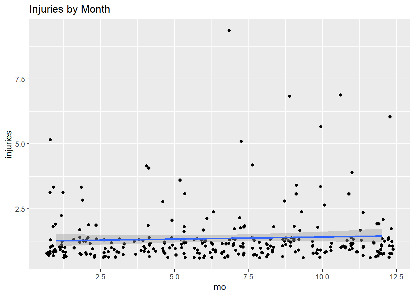

Fit a poisson regression in R using glm(formula, data, family = poisson). But first, check whether the mean and variance of injuries are the same magnitude? If not, then use family = quasipoisson.

mean(fire$injuries)

## [1] 1.4

var(fire$injuries)

## [1] 1

They are of the same magnitude, so fit the regression with family = poisson.

m2 <- glm(injuries ~ mo, family = poisson, data = fire)
summary(m2)

## 
## Call:
## glm(formula = injuries ~ mo, family = poisson, data = fire)
## 
## Deviance Residuals: 
##    Min      1Q  Median      3Q     Max  
## -0.399  -0.347  -0.303  -0.250   4.318  
## 
## Coefficients:
##             Estimate Std. Error z value Pr(>|z|)  
## (Intercept)   0.2280     0.1048    2.18     0.03 *
## mo            0.0122     0.0140    0.87     0.38  
## ---
## Signif. codes:  0 '***' 0.001 '**' 0.01 '*' 0.05 '.' 0.1 ' ' 1
## 
## (Dispersion parameter for poisson family taken to be 1)
## 
##     Null deviance: 139.87  on 299  degrees of freedom
## Residual deviance: 139.11  on 298  degrees of freedom
## AIC: 792.1
## 
## Number of Fisher Scoring iterations: 5

The predicted value \(\hat{y}\) is the estimated log of the response variable,

\[\hat{y} = X \hat{\beta} = \ln (\lambda).\]

Suppose mo is January (mo = ), then the log ofinjuries` is \(\hat{y} = 0.323787\). Or, more intuitively, the expected count of injuries is \(\exp(0.323787) = 1.38\)

predict(m2, newdata = data.frame(mo=1))

##    1 
## 0.24

predict(m2, newdata = data.frame(mo=1), type = "response")

##   1 
## 1.3

Here is a plot of the predicted counts in red.

augment(m2, type.predict = "response") %>%
  ggplot(aes(x = mo, y = injuries)) +
  geom_point() +
  geom_point(aes(y = .fitted), color = "red") + 
  scale_y_continuous(limits = c(0, NA)) +
  labs(x = "Month",
       y = "Injuries",
       title = "Poisson Fitted Line Plot")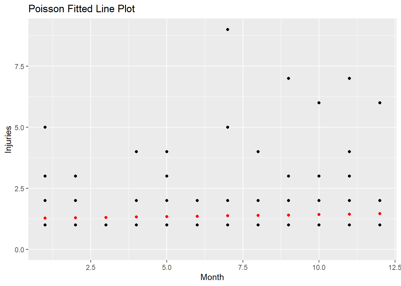

Evaluate a logistic model fit with an analysis of deviance.

(perf <- glance(m2))

## # A tibble: 1 x 7
##   null.deviance df.null logLik   AIC   BIC deviance df.residual
##           <dbl>   <int>  <dbl> <dbl> <dbl>    <dbl>       <int>
## 1          140.     299  -394.  792.  799.     139.         298

(pseudoR2 <- 1 - perf$deviance / perf$null.deviance)

## [1] 0.0054

The deviance of the null model (no regressors) is 139.9. The deviance of the full model is 132.2. The psuedo-R2 is very low at .05. How about the RMSE?

RMSE(pred = predict(m2, type = "response"), obs = fire$injuries)

## [1] 1

The average prediction error is about 0.99. That’s almost as much as the variance of injuries - i.e., just predicting the mean of injuries would be almost as good! Use the GainCurvePlot() function to plot the gain curve.

augment(m2, type.predict = "response") %>%
  ggplot(aes(x = injuries, y = .fitted)) +
  geom_point() +
  geom_smooth(method ="lm") +
  labs(x = "Actual",
       y = "Predicted",
       title = "Poisson Fitted vs Actual")

## `geom_smooth()` using formula 'y ~ x'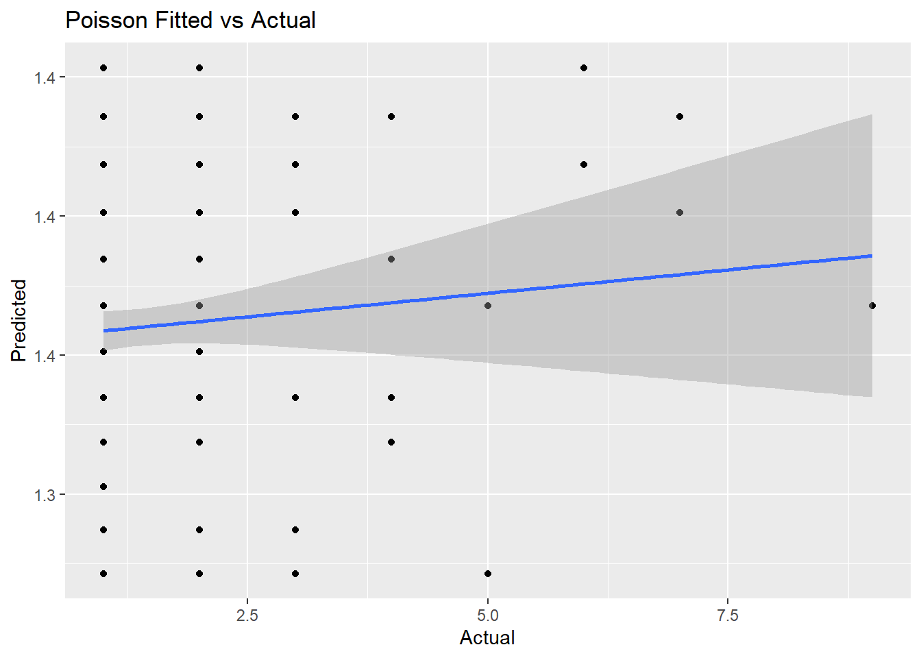

augment(m2) %>% data.frame() %>% 
  GainCurvePlot(xvar = ".fitted", truthVar = "injuries", title = "Poisson Model")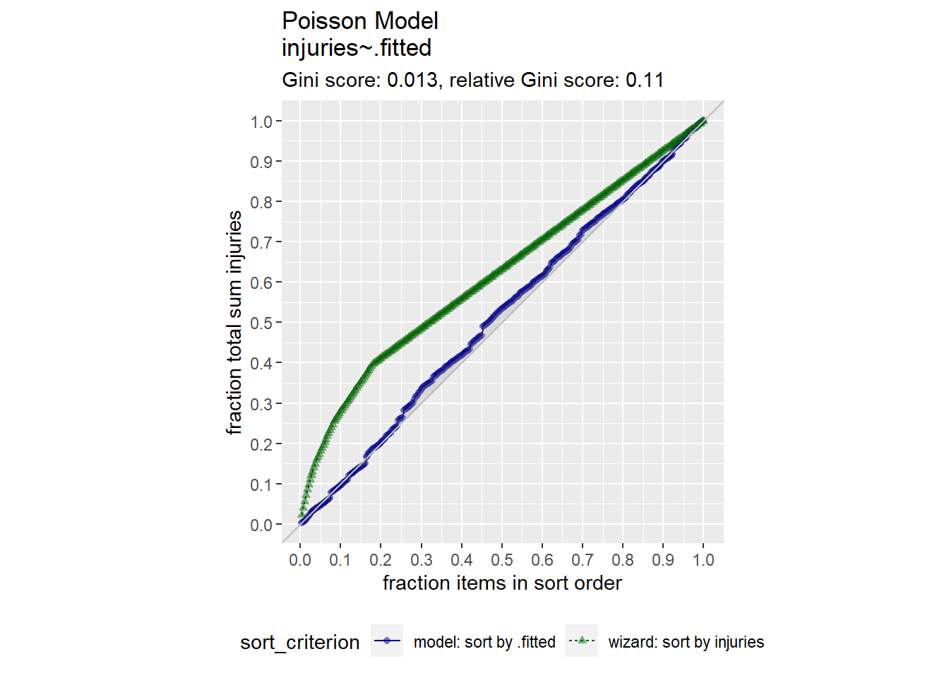

It seems that mo was a poor predictor of injuries.