4.6 Interpretation
A plot of the standardized coefficients shows the relative importance of each variable. The distance the coefficients are from zero shows how much a change in a standard deviation of the regressor changes the mean of the predicted value. The CI shows the precision. The plot shows not only which variables are significant, but also which are important.
d_sc <- d %>% mutate_at(c("mpg", "disp", "hp", "drat", "wt", "qsec"), scale)
m_sc <- lm(mpg ~ ., d_sc[,1:9])
lm_summary <- summary(m_sc)$coefficients
df <- data.frame(Features = rownames(lm_summary),
                 Estimate = lm_summary[,'Estimate'],
                 std_error = lm_summary[,'Std. Error'])
df$lower = df$Estimate - qt(.05/2, m_sc$df.residual) * df$std_error
df$upper = df$Estimate + qt(.05/2, m_sc$df.residual) * df$std_error
df <- df[df$Features != "(Intercept)",]

ggplot(df) +
  geom_vline(xintercept = 0, linetype = 4) +
  geom_point(aes(x = Estimate, y = Features)) +
  geom_segment(aes(y = Features, yend = Features, x=lower, xend=upper),
               arrow = arrow(angle=90, ends='both', length = unit(0.1, 'cm'))) +
  scale_x_continuous("Standardized Weight") +
  labs(title = "Model Feature Importance")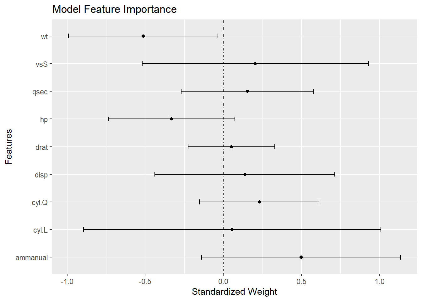
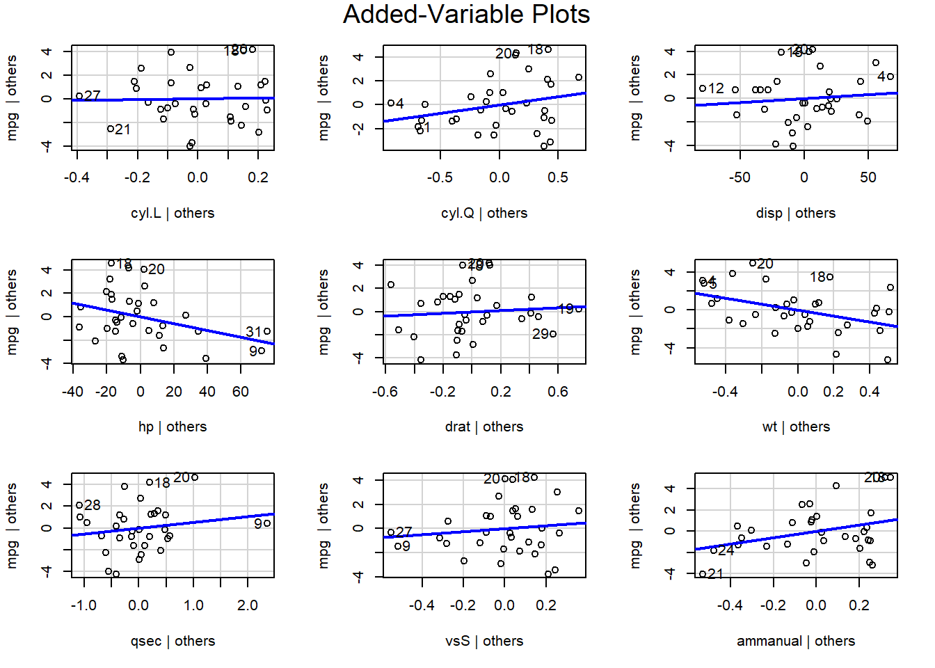
The added variable plot shows the bivariate relationship between \(Y\) and \(X_i\) after accounting for the other variables. For example, the partial regression plots of y ~ x1 + x2 + x3 would plot the residuals of y ~ x2 + x3 vs x1, and so on.