11.2 HCA
Hierarchical clustering (also called hierarchical cluster analysis or HCA) is a method of cluster analysis which builds a hierarchy of clusters (usually presented in a dendrogram). The HCA process is:
Calculate the distance between each observation with
dist()ordaisy(). We did that above when we createddat_2_gwr.Cluster the two closest observations into a cluster with
hclust(). Then calculate the cluster’s distance to the remaining observations. If the shortest distance is between two observations, define a second cluster, otherwise adds the observation as a new level to the cluster. The process repeats until all observations belong to a single cluster. The “distance” to a cluster can be defined as:
- complete: distance to the furthest member of the cluster,
- single: distance to the closest member of the cluster,
- average: average distance to all members of the cluster, or
- centroid: distance between the centroids of each cluster.
Complete and average distances tend to produce more balanced trees and are most common. Pruning an unbalanced tree can result in most observations assigned to one cluster and only a few observations assigned to other clusters. This is useful for identifying outliers.
- Evaluate the
hclusttree with a dendogram, principal component analysis (PCA), and/or summary statistics. The vertical lines in a dendogram indicate the distance between nodes and their associated cluster. Choose the number of clusters to keep by identifying a cut point that creates a reasonable number of clusters with a substantial number of observations per cluster (I know, “reasonable” and “substantial” are squishy terms). Below, cutting at height 0.65 to create 7 clusters seems good.
# Inspect the tree to choose a size.
plot(color_branches(as.dendrogram(mdl_hc), k = 7))
abline(h = .65, col = "red")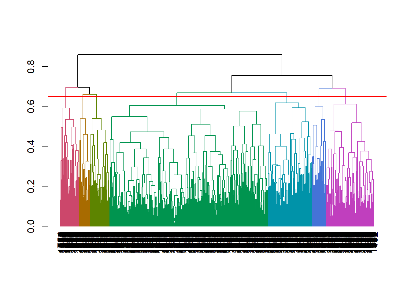
- “Cut” the hierarchical tree into the desired number of clusters (
k) or heighthwithcutree(hclust, k = NULL, h = NULL).cutree()returns a vector of cluster memberships. Attach this vector back to the original dataframe for visualization and summary statistics.
- Calculate summary statistics and draw conclusions. Useful summary statistics are typically membership count, and feature averages (or proportions).
## # A tibble: 7 x 8
##   cluster EmployeeNumber MonthlyIncome YearsAtCompany YearsWithCurrMa~
##     <int>          <dbl>         <dbl>          <dbl>            <dbl>
## 1       1          1051.         8056.           8.21             4.23
## 2       2          1029.         5146.           5.98             3.85
## 3       3           974.         4450.           5.29             3.51
## 4       4          1088.         3961.           4.60             2.64
## 5       5           980.        16534.          14.2              6.80
## 6       6          1036.        12952.          14.9              7.64
## 7       7           993.        13733.          12.8              6.53
## # ... with 3 more variables: TotalWorkingYears <dbl>, Age <dbl>,
## #   YearsInCurrentRole <dbl>
11.2.0.1 K-Means vs HCA
Hierarchical clustering has some advantages over k-means. It can use any distance method - not just euclidean. The results are stable - k-means can produce different results each time. While they can both be evaluated with the silhouette and elbow plots, hierachical clustering can also be evaluated with a dendogram. But hierarchical clusters has one significant drawback: it is computationally complex compared to k-means. For this last reason, k-means is more common.