Chapter 13 Text Mining
Text mining may be thought of as the process of distilling actionable insights from text, typically by identifying patterns with statistical pattern learning. Typical text mining tasks include text categorization, sentiment analysis, and topic modeling.
There are two approaches to text mining. Semantic parsing identifies words by type and order (sentences, phrases, nouns/verbs, proper nouns, etc.). Bag of Words treats words as simply attributes of the document. Bag of words is obviously the simpler way to go.
The qdap package provides parsing tools for preparing transcript data.
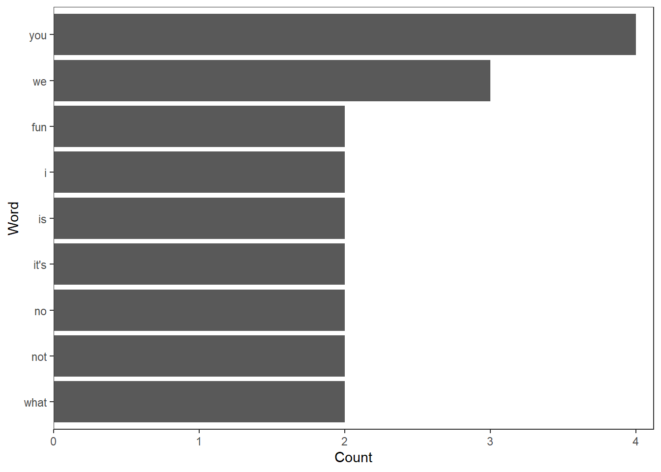
For example, freq_terms() parses text and counts the terms.
##   WORD FREQ
## 1 you     4
## 2 we      3
## 3 fun     2
## 4 i       2
## 5 is      2
## 6 it's    2
## 7 no      2
## 8 not     2
## 9 what    2
You can also plot the terms.

There are two kinds of the corpus data types, the permanent corpus, PCorpus, and the volatile corpus, VCorpus. The volatile corpus is held in RAM rather than saved to disk. Create a volatile corpus with tm::vCorpous(). vCorpous() takes either a text source created with tm::VectorSource() or a dataframe source created with Dataframe Source() where the input dataframe has cols doc_id, text_id and zero or more metadata columns.
tweets <- read_csv(file = "https://assets.datacamp.com/production/repositories/19/datasets/27a2a8587eff17add54f4ba288e770e235ea3325/coffee.csv")## Parsed with column specification:
## cols(
## num = col_double(),
## text = col_character(),
## favorited = col_logical(),
## replyToSN = col_character(),
## created = col_character(),
## truncated = col_logical(),
## replyToSID = col_double(),
## id = col_double(),
## replyToUID = col_double(),
## statusSource = col_character(),
## screenName = col_character(),
## retweetCount = col_double(),
## retweeted = col_logical(),
## longitude = col_logical(),
## latitude = col_logical()
## )coffee_tweets <- tweets$text
coffee_source <- VectorSource(coffee_tweets)
coffee_corpus <- VCorpus(coffee_source)
# Text of first tweet
coffee_corpus[[1]][1]## $content
## [1] "@ayyytylerb that is so true drink lots of coffee"In bag of words text mining, cleaning helps aggregate terms, especially words with common stems like “miner” and “mining”. There are several functions useful for preprocessing: tolower(), tm::removePunctuation(), tm::removeNumbers(), tm::stripWhiteSpace(), and removeWords(). Apply these functions to the documents in a VCorpus object with tm_map(). If the function is not one of the pre-defined functions, wrap it in content_transformer(). Another preprocessing function is stemDocument().
# Create the object: text
text <- "<b>She</b> woke up at       6 A.M. It\'s so early!  She was only 10% awake and began drinking coffee in front of her computer."
tolower(text)
## [1] "<b>she</b> woke up at 6 a.m. it's so early! she was only 10% awake and began drinking coffee in front of her computer."## [1] "bSheb woke up at 6 AM Its so early She was only 10 awake and began drinking coffee in front of her computer"## [1] "<b>She</b> woke up at A.M. It's so early! She was only % awake and began drinking coffee in front of her computer."## [1] "<b>She</b> woke up at 6 A.M. It's so early! She was only 10% awake and began drinking coffee in front of her computer."The qdap package offers other preprocessing functions.
text <- "<b>She</b> woke up at       6 A.M. It\'s so early!  She was only 10% awake and began drinking coffee in front of her computer."
bracketX(text)
## [1] "She woke up at 6 A.M. It's so early! She was only 10% awake and began drinking coffee in front of her computer."## [1] "<b>She</b> woke up at six A.M. It's so early! She was only ten% awake and began drinking coffee in front of her computer."## [1] "<b>She</b> woke up at 6 AM It's so early! She was only 10% awake and began drinking coffee in front of her computer."## [1] "<b>She</b> woke up at 6 A.M. it is so early! She was only 10% awake and began drinking coffee in front of her computer."## [1] "<b>She</b> woke up at 6 A.M. It's so early! She was only 10 percent awake and began drinking coffee in front of her computer."tm::stopwords("en") returns a vector of stop words. You can add to the list with concatenation.
## [1] "<b>She</b> woke 6 A.M. It's early! She 10% awake began drinking front computer."tm::stemDocument() and tm::stemCompletion() reduce the variation in terms.
complicate <- c("complicated", "complication", "complicatedly")

stem_doc <- stemDocument(complicate)

comp_dict <- c("complicate")

complete_text <- stemCompletion(stem_doc, comp_dict)
complete_text
## complic complic complic
## "complicate" "complicate" "complicate"clean_corpus <- function(corpus){
corpus <- tm_map(corpus, removePunctuation)
corpus <- tm_map(corpus, content_transformer(tolower))
corpus <- tm_map(corpus, removeWords, words = c(stopwords("en"), "coffee", "mug"))
corpus <- tm_map(corpus, stripWhitespace)
return(corpus)
}
clean_corp <- clean_corpus(coffee_corpus)
content(clean_corp[[1]])## [1] "ayyytylerb true drink lots "## [1] "@ayyytylerb that is so true drink lots of coffee"To perform the analysis of the tweets, convert the corpus into either a document term matrix (DTM, documents as rows, terms as cols), or a term document matrix (TDM, terms as rows, documents as cols).
## <<TermDocumentMatrix (terms: 3075, documents: 1000)>>
## Non-/sparse entries: 7384/3067616
## Sparsity           : 100%
## Maximal term length: 27
## Weighting          : term frequency (tf)
# Convert coffee_tdm to a matrix
coffee_m <- as.matrix(coffee_tdm)
# Print the dimensions of the matrix
dim(coffee_m)## [1] 3075 1000## Docs
## Terms 25 26 27 28 29 30 31 32 33 34 35
## star 0 0 0 0 0 0 0 0 0 0 0
## starbucks 0 1 1 0 0 0 0 0 0 1 0