8.4 Random Forests
Random forests improve bagged trees by way of a small tweak that de-correlates the trees. As in bagging, the algorithm builds a number of decision trees on bootstrapped training samples. But when building these decision trees, each time a split in a tree is considered, a random sample of mtry predictors is chosen as split candidates from the full set of p predictors. A fresh sample of mtry predictors is taken at each split. Typically \(mtry \sim \sqrt{p}\). Bagged trees are thus a special case of random forests where mtry = p.
8.4.0.1 Random Forest Classification Tree
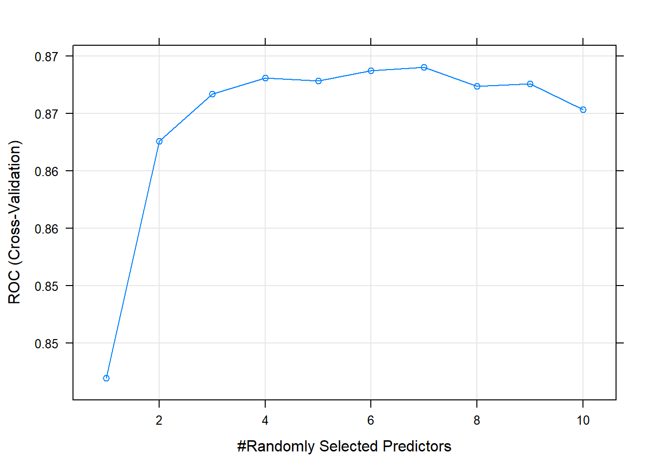
Now I’ll try it with the random forest method by specifying method = "rf". Hyperparameter mtry can take any value from 1 to 17 (the number of predictors) and I expect the best value to be near \(\sqrt{17} \sim 4\).
set.seed(1234)
oj_mdl_rf <- train(
   Purchase ~ .,
   data = oj_train,
   method = "rf",
   metric = "ROC",
   tuneGrid = expand.grid(mtry = 1:10), # searching around mtry=4
   trControl = oj_trControl
)
oj_mdl_rf
## Random Forest
##
## 857 samples
## 17 predictor
## 2 classes: 'CH', 'MM'
##
## No pre-processing
## Resampling: Cross-Validated (10 fold)
## Summary of sample sizes: 772, 772, 771, 770, 771, 771, ...
## Resampling results across tuning parameters:
##
## mtry ROC Sens Spec
## 1 0.84 0.90 0.55
## 2 0.86 0.88 0.70
## 3 0.87 0.86 0.72
## 4 0.87 0.85 0.72
## 5 0.87 0.85 0.71
## 6 0.87 0.84 0.73
## 7 0.87 0.84 0.72
## 8 0.87 0.84 0.72
## 9 0.87 0.83 0.72
## 10 0.87 0.84 0.72
##
## ROC was used to select the optimal model using the largest value.
## The final value used for the model was mtry = 7.The largest ROC score was at mtry = 7 - higher than I expected.
Use the model to make predictions on the test set.
oj_preds_rf <- bind_cols(
   predict(oj_mdl_rf, newdata = oj_test, type = "prob"),
   Predicted = predict(oj_mdl_rf, newdata = oj_test, type = "raw"),
   Actual = oj_test$Purchase
)

oj_cm_rf <- confusionMatrix(oj_preds_rf$Predicted, reference = oj_preds_rf$Actual)
oj_cm_rf
## Confusion Matrix and Statistics
##
## Reference
## Prediction CH MM
## CH 110 16
## MM 20 67
##
## Accuracy : 0.831
## 95% CI : (0.774, 0.879)
## No Information Rate : 0.61
## P-Value [Acc > NIR] : 0.0000000000023
##
## Kappa : 0.648
##
## Mcnemar's Test P-Value : 0.617
##
## Sensitivity : 0.846
## Specificity : 0.807
## Pos Pred Value : 0.873
## Neg Pred Value : 0.770
## Prevalence : 0.610
## Detection Rate : 0.516
## Detection Prevalence : 0.592
## Balanced Accuracy : 0.827
##
## 'Positive' Class : CH
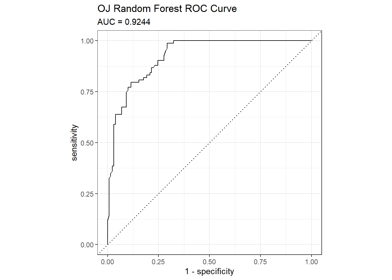
## The accuracy on the holdout set is 0.8310. The AUC is 0.9244. Here are the ROC and gain curves.
# AUC is 0.9190
mdl_auc <- Metrics::auc(actual = oj_preds_rf$Actual == "CH", oj_preds_rf$CH)
yardstick::roc_curve(oj_preds_rf, Actual, CH) %>%
  autoplot() +
  labs(
    title = "OJ Random Forest ROC Curve",
    subtitle = paste0("AUC = ", round(mdl_auc, 4))
  )
yardstick::gain_curve(oj_preds_rf, Actual, CH) %>%
  autoplot() +
  labs(title = "OJ Random Forest Gain Curve")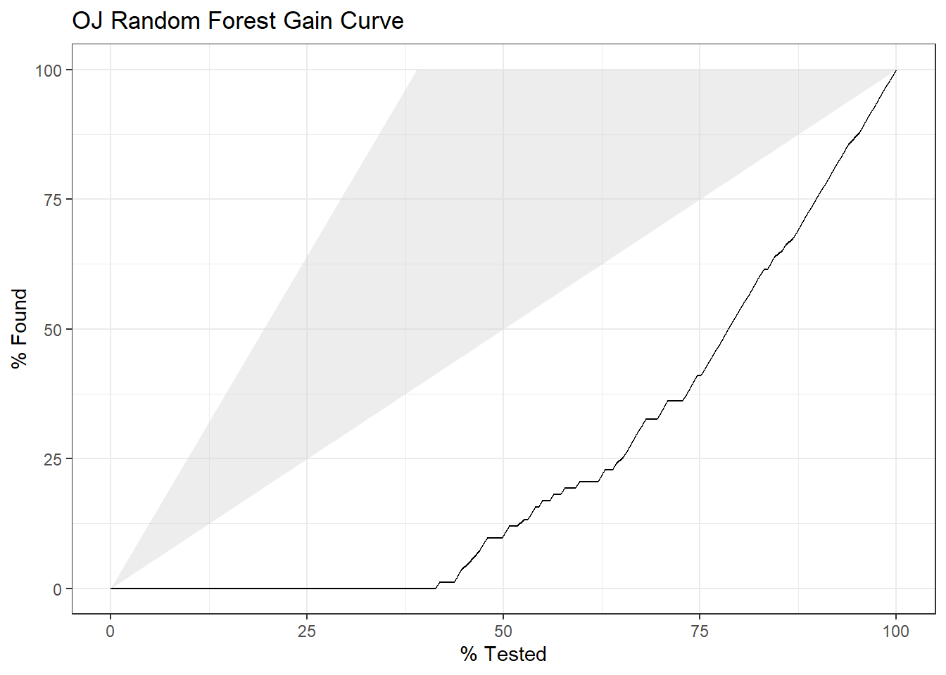
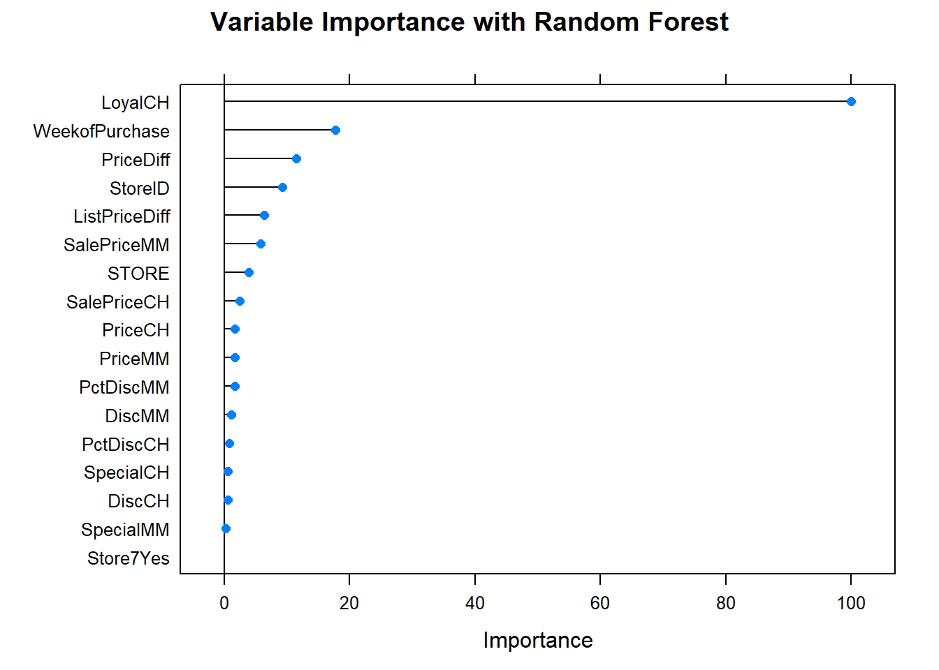
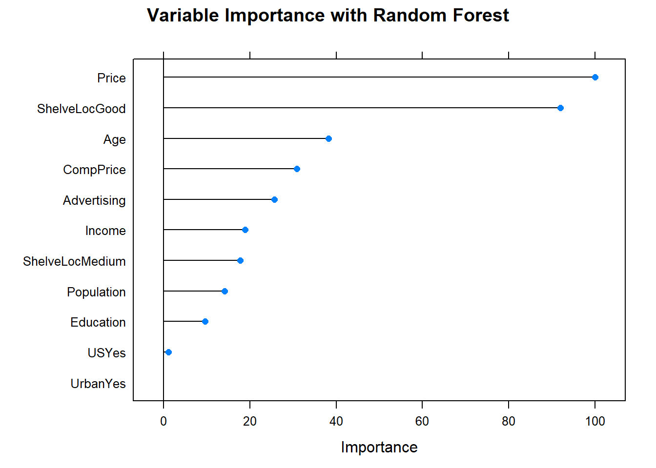
What are the most important variables?
Let’s update the scoreboard. The bagging and random forest models did pretty well, but the manual classification tree is still in first place. There’s still gradient boosting to investigate!
oj_scoreboard <- rbind(oj_scoreboard,
   data.frame(Model = "Random Forest", Accuracy = oj_cm_rf$overall["Accuracy"])
) %>% arrange(desc(Accuracy))
scoreboard(oj_scoreboard)
Model | Accuracy |
Single Tree | 0.8592 |
Single Tree (caret) | 0.8545 |
Bagging | 0.8451 |
Random Forest | 0.8310 |
8.4.0.2 Random Forest Regression Tree
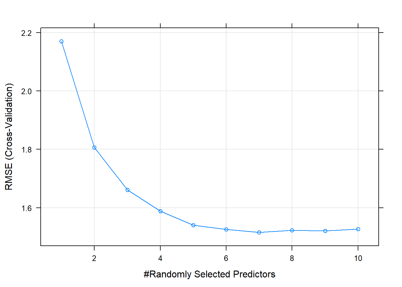
Now I’ll try it with the random forest method by specifying method = "rf". Hyperparameter mtry can take any value from 1 to 10 (the number of predictors) and I expect the best value to be near \(\sqrt{10} \sim 3\).
set.seed(1234)
cs_mdl_rf <- train(
   Sales ~ .,
   data = cs_train,
   method = "rf",
   tuneGrid = expand.grid(mtry = 1:10), # searching around mtry=3
   trControl = cs_trControl
)
cs_mdl_rf
## Random Forest
##
## 321 samples
## 10 predictor
##
## No pre-processing
## Resampling: Cross-Validated (10 fold)
## Summary of sample sizes: 289, 289, 289, 289, 289, 289, ...
## Resampling results across tuning parameters:
##
## mtry RMSE Rsquared MAE
## 1 2.2 0.64 1.7
## 2 1.8 0.73 1.4
## 3 1.7 0.75 1.3
## 4 1.6 0.75 1.3
## 5 1.5 0.76 1.2
## 6 1.5 0.75 1.2
## 7 1.5 0.75 1.2
## 8 1.5 0.75 1.2
## 9 1.5 0.74 1.2
## 10 1.5 0.74 1.2
##
## RMSE was used to select the optimal model using the smallest value.
## The final value used for the model was mtry = 7.The minimum RMSE is at mtry = 7.
Make predictions on the test set. Like the bagged tree model, this one also over-predicts at low end of Sales and under-predicts at high end. The RMSE of 1.7184 is better than bagging’s 1.9185.
cs_preds_rf <- bind_cols(
   Predicted = predict(cs_mdl_rf, newdata = cs_test),
   Actual = cs_test$Sales
)
(cs_rmse_rf <- RMSE(pred = cs_preds_rf$Predicted, obs = cs_preds_rf$Actual))
## [1] 1.7cs_preds_rf %>%
ggplot(aes(x = Actual, y = Predicted)) +
geom_point(alpha = 0.6, color = "cadetblue") +
geom_smooth(method = "loess", formula = "y ~ x") +
geom_abline(intercept = 0, slope = 1, linetype = 2) +
labs(title = "Carseats Random Forest, Predicted vs Actual (caret)")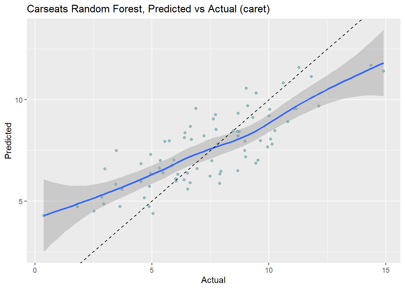
Let’s check in with the scoreboard.
cs_scoreboard <- rbind(cs_scoreboard,
   data.frame(Model = "Random Forest", RMSE = cs_rmse_rf)
) %>% arrange(RMSE)
scoreboard(cs_scoreboard)
Model | RMSE |
Random Forest | 1.7184 |
Bagging | 1.9185 |
Single Tree (caret) | 2.2983 |
Single Tree | 2.3632 |
The bagging and random forest models did very well - they took over the top positions!