7.3 Elastic Net

Elastic Net combines the penalties of ridge and lasso to get the best of both worlds. The loss function for elastic net is

\[L = \frac{\sum_{i = 1}^n \left(y_i - x_i^{'} \hat\beta \right)^2}{2n} + \lambda \frac{1 - \alpha}{2}\sum_{j=1}^k \hat{\beta}_j^2 + \lambda \alpha\left| \hat{\beta}_j \right|.\]

In this loss function, new parameter \(\alpha\) is a “mixing” parameter that balances the two approaches. If \(\alpha\) is zero, you are back to ridge regression, and if \(\alpha\) is one, you are back to lasso.

Example

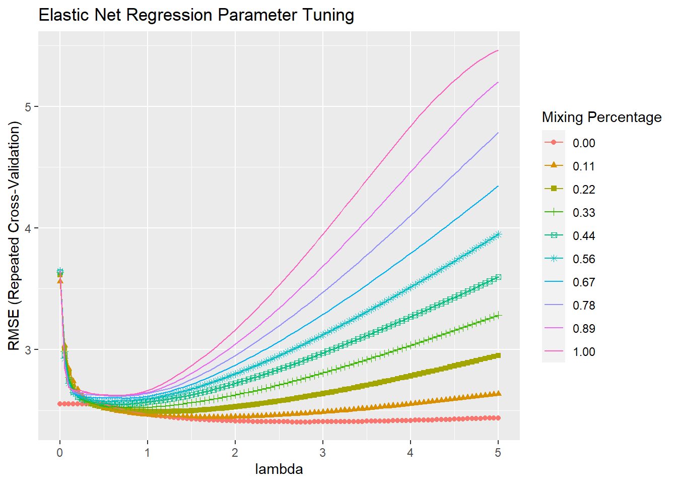
Continuing with prediction of mpg from the other variables in the mtcars data set, follow the same steps as before, but with elastic net regression there are two parameters to optimize: \(\lambda\) and \(\alpha\).

set.seed(1234)
mdl_elnet <- train(
  mpg ~ .,
  data = training,
  method = "glmnet",
  metric = "RMSE",
  preProcess = c("center", "scale"),
  tuneGrid = expand.grid(
    .alpha = seq(0, 1, length.out = 10),  # optimize an elnet regression
    .lambda = seq(0, 5, length.out = 101)
  ),
  trControl = train_control
  )

## Warning in nominalTrainWorkflow(x = x, y = y, wts = weights, info = trainInfo, :
## There were missing values in resampled performance measures.

mdl_elnet$bestTune

##    alpha lambda
## 56     0    2.8

The optimal tuning values (at the mininum RMSE) were alpha = 0.0 and lambda = 2.75, so the mix is 100% ridge, 0% lasso. You can see the RMSE minimum on the the plot. Alpha is on the horizontal axis and the different lambdas are shown as separate series.

ggplot(mdl_elnet) +
  labs(title = "Elastic Net Regression Parameter Tuning", x = "lambda")

## Warning: The shape palette can deal with a maximum of 6 discrete values because
## more than 6 becomes difficult to discriminate; you have 10. Consider
## specifying shapes manually if you must have them.

## Warning: Removed 404 rows containing missing values (geom_point).