8.6 Summary
I created four classification trees using the ISLR::OJ data set and four regression trees using the ISLR::Carseats data set. Let’s compare their performance.
8.6.1 Classification Trees
The caret::resamples() function summarizes the resampling performance on the final model produced in train(). It creates summary statistics (mean, min, max, etc.) for each performance metric (ROC, RMSE, etc.) for a list of models.
oj_resamples <- resamples(list("Single Tree (caret)" = oj_mdl_cart2,
                               "Bagged" = oj_mdl_bag,
                               "Random Forest" = oj_mdl_rf,
                               "GBM" = oj_mdl_gbm,
                               "XGBoost" = oj_mdl_xgb))
summary(oj_resamples)
##
## Call:
## summary.resamples(object = oj_resamples)
##
## Models: Single Tree (caret), Bagged, Random Forest, GBM, XGBoost
## Number of resamples: 10
##
## ROC
## Min. 1st Qu. Median Mean 3rd Qu. Max. NA's
## Single Tree (caret) 0.74 0.84 0.86 0.85 0.88 0.92 0
## Bagged 0.79 0.84 0.86 0.86 0.88 0.89 0
## Random Forest 0.80 0.87 0.88 0.87 0.89 0.91 0
## GBM 0.82 0.87 0.91 0.89 0.91 0.94 0
## XGBoost 0.82 0.88 0.90 0.89 0.92 0.94 0
##
## Sens
## Min. 1st Qu. Median Mean 3rd Qu. Max. NA's
## Single Tree (caret) 0.77 0.85 0.85 0.86 0.89 0.92 0
## Bagged 0.77 0.83 0.83 0.84 0.85 0.92 0
## Random Forest 0.79 0.83 0.83 0.84 0.85 0.92 0
## GBM 0.79 0.85 0.87 0.86 0.88 0.88 0
## XGBoost 0.81 0.87 0.89 0.88 0.90 0.92 0
##
## Spec
## Min. 1st Qu. Median Mean 3rd Qu. Max. NA's
## Single Tree (caret) 0.61 0.63 0.76 0.73 0.82 0.85 0
## Bagged 0.62 0.67 0.71 0.72 0.76 0.82 0
## Random Forest 0.58 0.65 0.74 0.72 0.81 0.85 0
## GBM 0.61 0.68 0.79 0.76 0.84 0.91 0
## XGBoost 0.61 0.64 0.78 0.75 0.82 0.88 0The mean ROC value is the performance measure I used to evaluate the models in train() (you can compare the Mean column to each model’s object (e.g., print(oj_mdl_cart2))). The best performing model on resamples based on the mean ROC score was XGBoost. It also had the highest mean sensitivity. GBM had the highest specificity. Here is a box plot of the distributions.
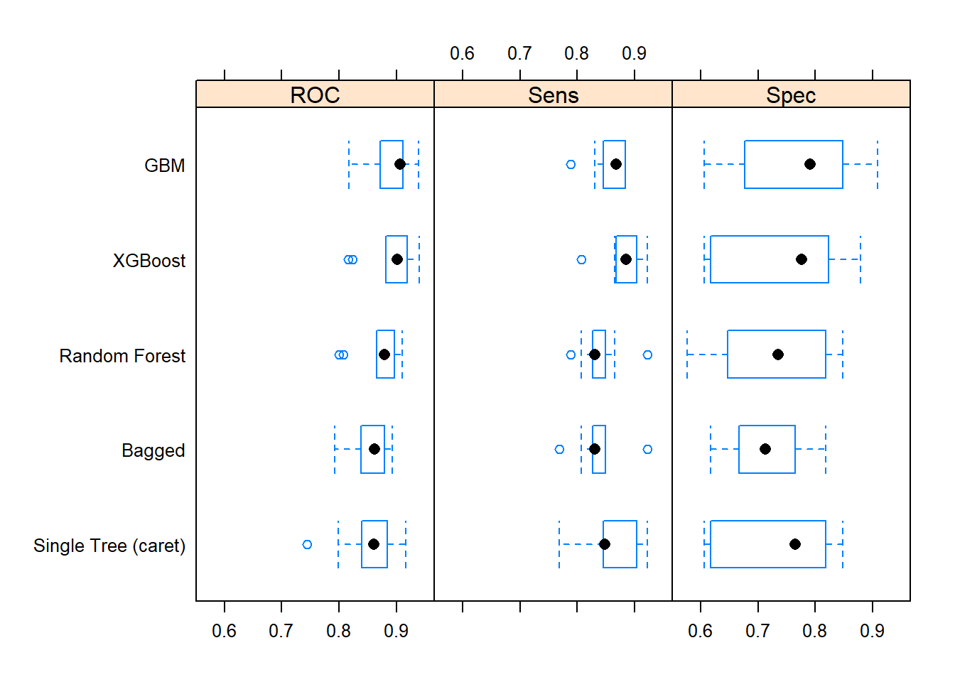
One way to evaluate the box plots is with a post-hoc test of differences. The single tree was about the same as the random forest and bagged models. GBM and XGBoost were also statistically equivalent.
##
## Call:
## diff.resamples(x = oj_resamples)
##
## Models: Single Tree (caret), Bagged, Random Forest, GBM, XGBoost
## Metrics: ROC, Sens, Spec
## Number of differences: 10
## p-value adjustment: bonferroni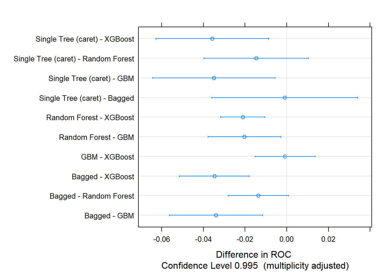
8.6.2 Regression Trees
Here is the summary of resampling metrics for the Carseats models.
cs_resamples <- resamples(list("Single Tree (caret)" = cs_mdl_cart2,
                               "Bagged" = cs_mdl_bag,
                               "Random Forest" = cs_mdl_rf,
                               "GBM" = cs_mdl_gbm,
                               "XGBoost" = cs_mdl_xgb))
summary(cs_resamples)
##
## Call:
## summary.resamples(object = cs_resamples)
##
## Models: Single Tree (caret), Bagged, Random Forest, GBM, XGBoost
## Number of resamples: 10
##
## MAE
## Min. 1st Qu. Median Mean 3rd Qu. Max. NA's
## Single Tree (caret) 1.37 1.59 1.73 1.70 1.80 2.1 0
## Bagged 0.93 1.13 1.35 1.34 1.57 1.7 0
## Random Forest 0.85 1.04 1.26 1.21 1.39 1.5 0
## GBM 0.72 0.86 0.92 0.94 1.04 1.1 0
## XGBoost 0.66 0.79 0.90 0.88 0.96 1.1 0
##
## RMSE
## Min. 1st Qu. Median Mean 3rd Qu. Max. NA's
## Single Tree (caret) 1.69 1.90 2.0 2.1 2.2 2.5 0
## Bagged 1.21 1.41 1.7 1.7 2.0 2.1 0
## Random Forest 1.07 1.28 1.6 1.5 1.7 1.9 0
## GBM 0.93 1.08 1.2 1.2 1.3 1.4 0
## XGBoost 0.86 0.98 1.1 1.1 1.2 1.3 0
##
## Rsquared
## Min. 1st Qu. Median Mean 3rd Qu. Max. NA's
## Single Tree (caret) 0.39 0.50 0.52 0.50 0.53 0.59 0
## Bagged 0.53 0.63 0.68 0.68 0.73 0.78 0
## Random Forest 0.68 0.70 0.76 0.75 0.80 0.83 0
## GBM 0.82 0.83 0.85 0.85 0.86 0.87 0
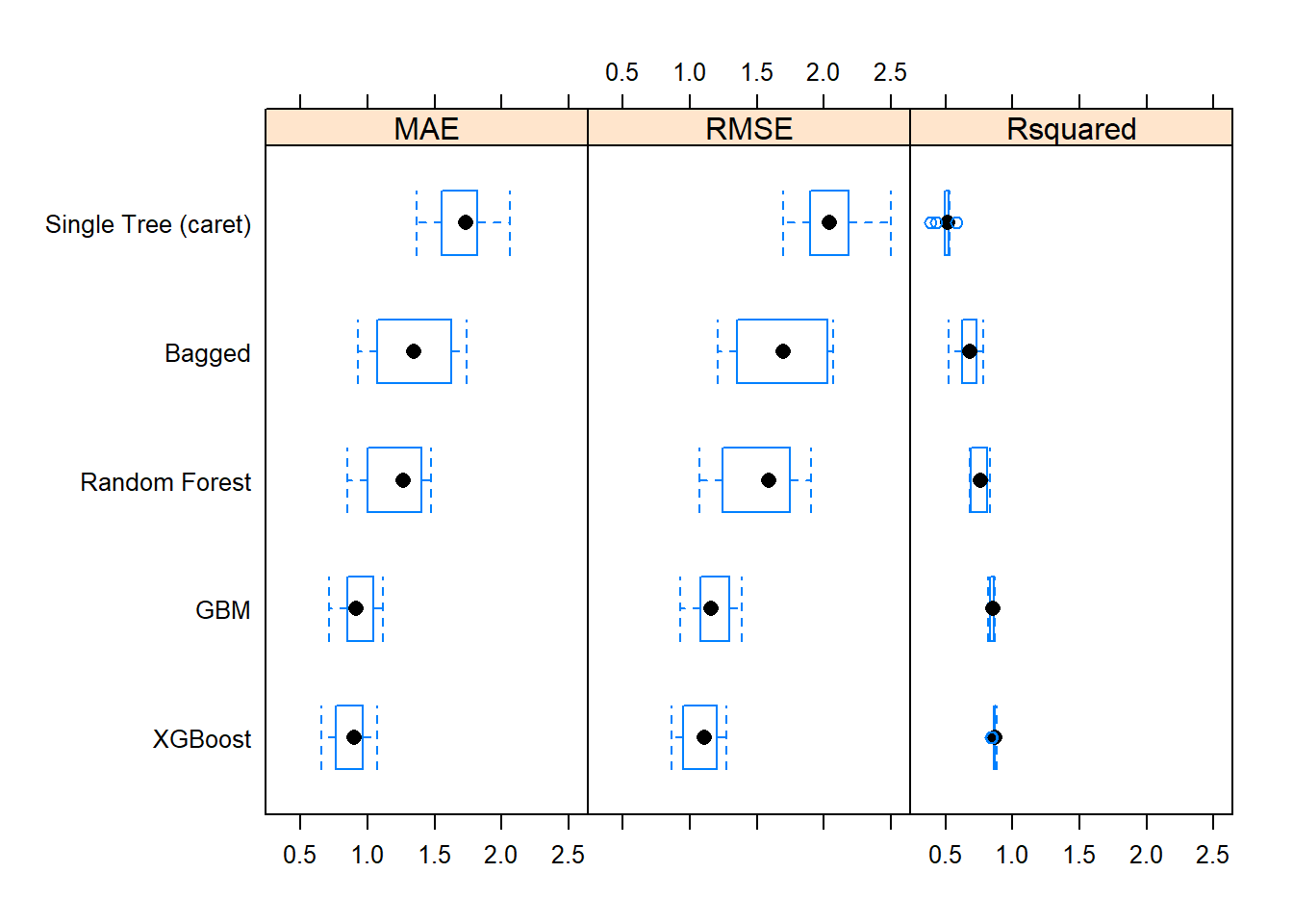
## XGBoost 0.84 0.86 0.87 0.86 0.87 0.88 0The best performing model on resamples based on the mean RMSE score was XGBoost. It also had the lowest mean absolute error (MAE) and highest R-squared. Here is a box plot of the distributions.
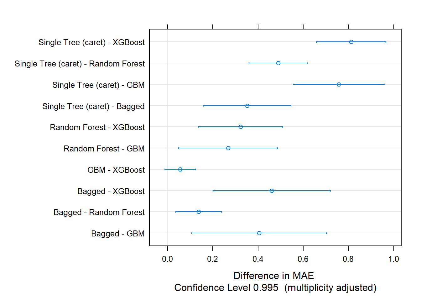
The post-hoc test indicates all models differed from each other except for GBM and XGBoost.
##
## Call:
## diff.resamples(x = cs_resamples)
##
## Models: Single Tree (caret), Bagged, Random Forest, GBM, XGBoost
## Metrics: MAE, RMSE, Rsquared
## Number of differences: 10
## p-value adjustment: bonferroni