16.1 N-Grams
Create n-grams by specifying unnest_tokens(..., token = "ngrams", n) where n = 2 is a bigram, etc. To remove the stop words, separate the n-grams, then filter on the stop_words data set.
austin.2gram <- austen_books() %>%
  group_by(book) %>%
  mutate(linenumber = row_number(),
         chapter = cumsum(str_detect(text, regex("^chapter [\\divxlc]",
                                                 ignore_case = TRUE)))) %>%
  ungroup() %>%
  unnest_tokens(output = bigram, input = text, token = "ngrams", n = 2)

austin.2gram <- austin.2gram %>%
  separate(bigram, c("word1", "word2"), sep = " ") %>%
  filter(!word1 %in% stop_words$word &
           !word2 %in% stop_words$word &
           !is.na(word1) & !is.na(word2)) %>%
  unite(bigram, word1, word2, sep = " ")

austin.2gram %>%
  count(book, bigram, sort = TRUE)
## # A tibble: 31,391 x 3
## book bigram n
## <fct> <chr> <int>
## 1 Mansfield Park sir thomas 266
## 2 Mansfield Park miss crawford 196
## 3 Emma miss woodhouse 143
## 4 Persuasion captain wentworth 143
## 5 Emma frank churchill 114
## 6 Persuasion lady russell 110
## 7 Persuasion sir walter 108
## 8 Mansfield Park lady bertram 101
## 9 Emma miss fairfax 98
## 10 Sense & Sensibility colonel brandon 96
## # ... with 31,381 more rowsHere are the most commonly mentioned streets in Austin’s novels.
austin.2gram %>%
  separate(bigram, c("word1", "word2"), sep = " ") %>%
  filter(word2 == "street") %>%
  count(book, word1, sort = TRUE)
## # A tibble: 33 x 3
## book word1 n
## <fct> <chr> <int>
## 1 Sense & Sensibility harley 16
## 2 Sense & Sensibility berkeley 15
## 3 Northanger Abbey milsom 10
## 4 Northanger Abbey pulteney 10
## 5 Mansfield Park wimpole 9
## 6 Pride & Prejudice gracechurch 8
## 7 Persuasion milsom 5
## 8 Sense & Sensibility bond 4
## 9 Sense & Sensibility conduit 4
## 10 Persuasion rivers 4
## # ... with 23 more rowsBind the tf-idf statistics. Tf-idf is short for term frequency–inverse document frequency. It is a statistic that indicates how important a word is to a document in a collection or corpus. Tf–idf increases with the number of times a word appears in the document and decreases with the number of documents in the corpus that contain the word. The idf adjusts for the fact that some words appear more frequently in general.
austen_books() %>%
  group_by(book) %>%
  mutate(linenumber = row_number(),
         chapter = cumsum(str_detect(text, regex("^chapter [\\divxlc]",
                                                 ignore_case = TRUE)))) %>%
  ungroup() %>%
  unnest_tokens(output = bigram, input = text, token = "ngrams", n = 2) %>%
  separate(bigram, c("word1", "word2"), sep = " ") %>%
  filter(!word1 %in% stop_words$word &
           !word2 %in% stop_words$word &
           !is.na(word1) & !is.na(word2)) %>%
  unite(bigram, word1, word2, sep = " ")
## # A tibble: 38,913 x 4
## book linenumber chapter bigram
## <fct> <int> <int> <chr>
## 1 Sense & Sensibility 3 0 jane austen
## 2 Sense & Sensibility 10 1 chapter 1
## 3 Sense & Sensibility 14 1 norland park
## 4 Sense & Sensibility 17 1 surrounding acquaintance
## 5 Sense & Sensibility 17 1 late owner
## 6 Sense & Sensibility 18 1 advanced age
## 7 Sense & Sensibility 19 1 constant companion
## 8 Sense & Sensibility 20 1 happened ten
## 9 Sense & Sensibility 22 1 henry dashwood
## 10 Sense & Sensibility 23 1 norland estate
## # ... with 38,903 more rowsaustin.2gram %>%
count(book, bigram) %>%
bind_tf_idf(bigram, book, n) %>%
group_by(book) %>%
top_n(n = 10, wt = tf_idf) %>%
ggplot(aes(x = fct_reorder(bigram, n), y = tf_idf, fill = book)) +
geom_col(show.legend = FALSE) +
facet_wrap(~book, scales = "free_y", ncol = 2) +
labs(y = "tf-idf of bigram to novel") +
coord_flip() 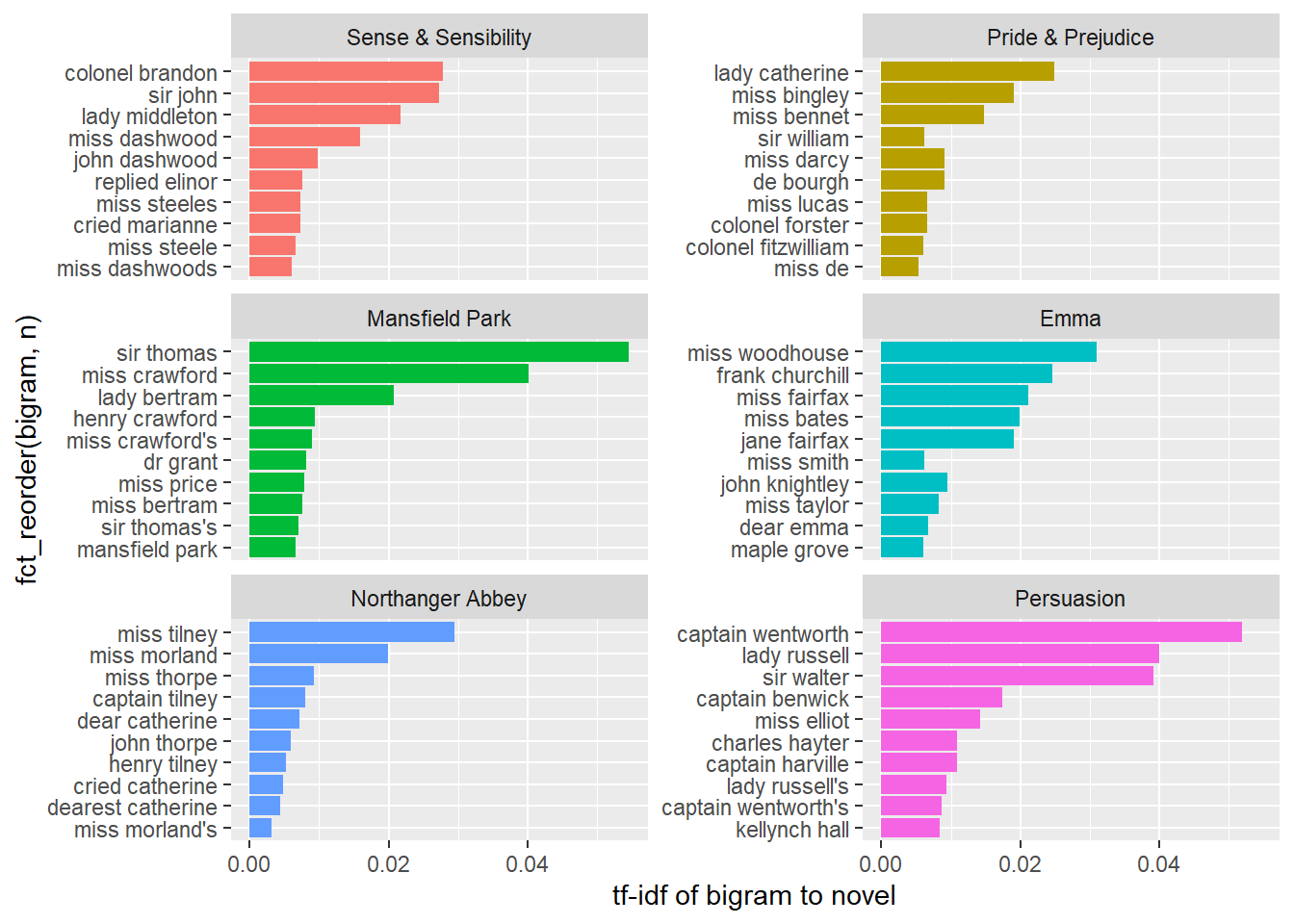
A good way to visualize bigrams is with a network graph. Packages igraph and ggraph provides tools for this purpose.
set.seed(2016)

austen_books() %>%
  group_by(book) %>%
  mutate(linenumber = row_number(),
         chapter = cumsum(str_detect(text, regex("^chapter [\\divxlc]",
                                                 ignore_case = TRUE)))) %>%
  ungroup() %>%
  unnest_tokens(output = bigram, input = text, token = "ngrams", n = 2) %>%
  separate(bigram, c("word1", "word2"), sep = " ") %>%
  filter(!word1 %in% stop_words$word &
           !word2 %in% stop_words$word &
           !is.na(word1) & !is.na(word2)) %>%
  count(word1, word2) %>%
  filter(n > 20) %>%
  graph_from_data_frame() %>%  # creates unformatted "graph"
  ggraph(layout = "fr") +
  geom_edge_link(aes(edge_alpha = n),
                 show.legend = FALSE,
                 arrow = grid::arrow(type = "closed",
                                     length = unit(.15, "inches")),
                 end_cap = circle(.07, 'inches')) +
  geom_node_point(color = "lightblue",
                  size = 5) +
  geom_node_text(aes(label = name), vjust = 1, hjust = 1) +
  theme_void()
If you want to count the number of times that two words appear within the same document, or to see how correlated they are, widen the data with the widyr package.
austen_books() %>%
  filter(book == "Pride & Prejudice") %>%
  mutate(section = row_number() %/% 10) %>%
  filter(section > 0) %>%
  unnest_tokens(word, text) %>%
  filter(!word %in% stop_words$word) %>%
  pairwise_count(word, section, sort = TRUE)
## Warning: `distinct_()` is deprecated as of dplyr 0.7.0.
## Please use `distinct()` instead.
## See vignette('programming') for more help
## This warning is displayed once every 8 hours.
## Call `lifecycle::last_warnings()` to see where this warning was generated.## Warning: `tbl_df()` is deprecated as of dplyr 1.0.0.
## Please use `tibble::as_tibble()` instead.
## This warning is displayed once every 8 hours.
## Call `lifecycle::last_warnings()` to see where this warning was generated.## # A tibble: 796,008 x 3
## item1 item2 n
## <chr> <chr> <dbl>
## 1 darcy elizabeth 144
## 2 elizabeth darcy 144
## 3 miss elizabeth 110
## 4 elizabeth miss 110
## 5 elizabeth jane 106
## 6 jane elizabeth 106
## 7 miss darcy 92
## 8 darcy miss 92
## 9 elizabeth bingley 91
## 10 bingley elizabeth 91
## # ... with 795,998 more rowsThe correlation among words is how often they appear together relative to how often they appear separately. The phi coefficient is defined
\[\phi = \frac{n_{11}n_{00} - n_{10}n_{01}}{\sqrt{n_{1.}n_{0.}n_{.1}n_{.0}}}\]
where \(n_{10}\) means number of times section has word x, but not word y, and \(n_{1.}\) means total times section has word x. This lets us pick particular interesting words and find the other words most associated with them.
austen_books() %>%
  filter(book == "Pride & Prejudice") %>%
  mutate(section = row_number() %/% 10) %>%
  filter(section > 0) %>%
  unnest_tokens(word, text) %>%
  filter(!word %in% stop_words$word) %>%
  pairwise_cor(word, section, sort = TRUE) %>%
  filter(item1 %in% c("elizabeth", "pounds", "married", "pride")) %>%
  group_by(item1) %>%
  top_n(n = 4) %>%
  ungroup() %>%
  mutate(item2 = reorder(item2, correlation)) %>%
  ggplot(aes(x = item2, y = correlation)) +
  geom_bar(stat = "identity") +
  facet_wrap(~ item1, scales = "free") +
  coord_flip()
## Selecting by correlation
You can use the correlation to set a threshold for a graph.
set.seed(2016)

austen_books() %>%
  filter(book == "Pride & Prejudice") %>%
  mutate(section = row_number() %/% 10) %>%
  filter(section > 0) %>%
  unnest_tokens(word, text) %>%
  filter(!word %in% stop_words$word) %>%
  # filter to relatively common words
  group_by(word) %>%
  filter(n() > 20) %>%
  pairwise_cor(word, section, sort = TRUE) %>%
  filter(correlation > .15) %>%  # relatively correlated words
  graph_from_data_frame() %>%
  ggraph(layout = "fr") +
  geom_edge_link(aes(edge_alpha = correlation), show.legend = FALSE) +
  geom_node_point(color = "lightblue", size = 5) +
  geom_node_text(aes(label = name), repel = TRUE) +
  theme_void()