16.2 Converting to and from non-tidy formats
One of the most common objects in text mining packages is the document term matrix (DTM) where each row is a document, each column a term, and each value an appearance count. The broom package contains functions to convert between DTM and tidy formats.
Convert a DTM object into a tidy data frame with tidy(). Convert a tidy object into a sparse matrix with cast_sparse(), into a DTM with cast_dtm(), and into a “dfm” for quanteda with cast_dfm().
## <<DocumentTermMatrix (documents: 2246, terms: 10473)>>
## Non-/sparse entries: 302031/23220327
## Sparsity           : 99%
## Maximal term length: 18
## Weighting : term frequency (tf)## [1] "aaron" "abandon" "abandoned" "abandoning" "abbott"
## [6] "abboud"Create a tidy version of AssociatedPress with tidy().
ap_td <- tidy(AssociatedPress)
ap_td %>%
  inner_join(get_sentiments("bing"), by = c(term = "word")) %>%
  count(sentiment, term, wt = count) %>%
  ungroup() %>%
  filter(n >= 200) %>%
  mutate(n = ifelse(sentiment == "negative", -n, n)) %>%
  arrange(n) %>%
  ggplot(aes(x = fct_inorder(term), y = n, fill = sentiment)) +
  geom_bar(stat = "identity") +
  labs(title = "Most Common AP Sentiment Words",
       x = "",
       y = "Contribution to Sentiment") +
  theme(legend.position = "top",
        legend.title = element_blank()) +
  coord_flip()
The document-feature matrix dfm class from the quanteda text-mining package is another implementation of a document-term matrix. Here are the terms most specific (highest tf-idf) from each of four selected inaugural addresses.
data("data_corpus_inaugural", package = "quanteda")
inaug_dfm <- quanteda::dfm(data_corpus_inaugural, verbose = FALSE)
head(inaug_dfm)
## Document-feature matrix of: 6 documents, 9,360 features (93.8% sparse) and 4 docvars.
## features
## docs fellow-citizens of the senate and house representatives :
## 1789-Washington 1 71 116 1 48 2 2 1
## 1793-Washington 0 11 13 0 2 0 0 1
## 1797-Adams 3 140 163 1 130 0 2 0
## 1801-Jefferson 2 104 130 0 81 0 0 1
## 1805-Jefferson 0 101 143 0 93 0 0 0
## 1809-Madison 1 69 104 0 43 0 0 0
## features
## docs among vicissitudes
## 1789-Washington 1 1
## 1793-Washington 0 0
## 1797-Adams 4 0
## 1801-Jefferson 1 0
## 1805-Jefferson 7 0
## 1809-Madison 0 0
## [ reached max_nfeat ... 9,350 more features ]## # A tibble: 6 x 3
## document term count
## <chr> <chr> <dbl>
## 1 1789-Washington fellow-citizens 1
## 2 1797-Adams fellow-citizens 3
## 3 1801-Jefferson fellow-citizens 2
## 4 1809-Madison fellow-citizens 1
## 5 1813-Madison fellow-citizens 1
## 6 1817-Monroe fellow-citizens 5inaug_td %>%
bind_tf_idf(term = term, document = document, n = count) %>%
group_by(document) %>%
top_n(n = 10, wt = tf_idf) %>%
ungroup() %>%
filter(document %in% c("1861-Lincoln", "1933-Roosevelt", "1961-Kennedy", "2009-Obama")) %>%
arrange(document, desc(tf_idf)) %>%
ggplot(aes(x = fct_rev(fct_inorder(term)), y = tf_idf, fill = document)) +
geom_col() +
labs(x = "") +
theme(legend.position = "none") +
coord_flip() +
facet_wrap(~document, ncol = 2, scales = "free")
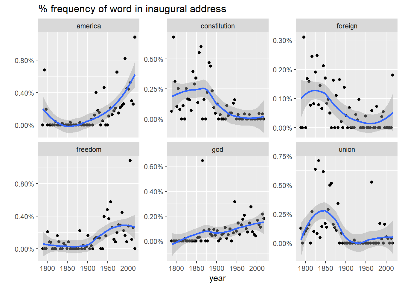
And here is word frequency trend ocer time for six selected terms.
inaug_td %>%
  extract(document, "year", "(\\d+)", convert = TRUE) %>%
  complete(year, term, fill = list(count = 0)) %>%
  group_by(year) %>%
  mutate(year_total = sum(count)) %>%
  filter(term %in% c("god", "america", "foreign", "union", "constitution", "freedom")) %>%
  ggplot(aes(x = year, y = count / year_total)) +
  geom_point() +
  geom_smooth() +
  facet_wrap(~ term, scales = "free_y") +
  scale_y_continuous(labels = scales::percent_format()) +
  labs(y = "",
       title = "% frequency of word in inaugural address")
## `geom_smooth()` using method = 'loess' and formula 'y ~ x'
Cast tidy data into document-term matrix with cast_dtm(), quanteda’s dfm with cast_dfm(), and sparese matrix with cast_sparse().
inaug_dtm <- cast_dtm(data = inaug_td, document = document, term = term, value = count)
inaug_dfm <- cast_dfm(data = inaug_td, document = document, term = term, value = count)
inaug_sparse <- cast_sparse(data = inaug_td, row = document, column = term, value = count)
An untokenized document collection is called a corpus. The corpuse may include metadata, such as ID, date/time, title, language, etc. Corpus metadata is usually stored as lists. Use tidy() to construct a table, one row per document.
## <<VCorpus>>
## Metadata:  corpus specific: 0, document level (indexed): 0
## Content: documents: 50## <<PlainTextDocument>>
## Metadata: 15
## Content: chars: 1287## # A tibble: 50 x 16
## author datetimestamp description heading id language origin topics
## <chr> <dttm> <chr> <chr> <chr> <chr> <chr> <chr>
## 1 <NA> 1987-02-26 10:18:06 "" COMPUT~ 10 en Reute~ YES
## 2 <NA> 1987-02-26 10:19:15 "" OHIO M~ 12 en Reute~ YES
## 3 <NA> 1987-02-26 10:49:56 "" MCLEAN~ 44 en Reute~ YES
## 4 By Ca~ 1987-02-26 10:51:17 "" CHEMLA~ 45 en Reute~ YES
## 5 <NA> 1987-02-26 11:08:33 "" <COFAB~ 68 en Reute~ YES
## 6 <NA> 1987-02-26 11:32:37 "" INVEST~ 96 en Reute~ YES
## 7 By Pa~ 1987-02-26 11:43:13 "" AMERIC~ 110 en Reute~ YES
## 8 <NA> 1987-02-26 11:59:25 "" HONG K~ 125 en Reute~ YES
## 9 <NA> 1987-02-26 12:01:28 "" LIEBER~ 128 en Reute~ YES
## 10 <NA> 1987-02-26 12:08:27 "" GULF A~ 134 en Reute~ YES
## # ... with 40 more rows, and 8 more variables: lewissplit <chr>,
## # cgisplit <chr>, oldid <chr>, places <named list>, people <lgl>, orgs <lgl>,
## # exchanges <lgl>, text <chr>