5.3 Exponential moving average (EMA)

EMA with \(n\) lagged period at time \(t\): \[\begin{align*} &ema_t(P,n)\\ &= \beta P_t + \beta (1-\beta)P_{t-1}+\beta(1-\beta )^{2}P_{t-2}+ \cdots\\ &=\beta P_t + (1-\beta) ema_{t-1}(P,n) \end{align*}\]

where the smoothing coefficient \(\beta\) is usually\[\beta=\frac{2}{n+1}\]

myEMA <- function (price,n){
  ema <- c()
  ema[1:(n-1)] <- NA
  ema[n]<- mean(price[1:n])
  beta <- 2/(n+1)
  for (i in (n+1):length(price)){
    ema[i]<-beta * price[i] + 
      (1-beta) * ema[i-1]
  }
  ema <- reclass(ema,price)
  return(ema)
}

Let us apply our function:

ema <-myEMA(Cl(AAPL),n=20)
tail(ema,n=3)

##                [,1]
## 2012-12-26 76.64302
## 2012-12-27 76.35131
## 2012-12-28 76.01295

In the application, the first EMA will be given by SMA, and subsequent EMAs is calcualted by the update formula.

5.3.1 TTR

In the TTR package, we can use EMA():

ema <-EMA(Cl(AAPL),n=20)
tail(ema,n=3)

##                 EMA
## 2012-12-26 76.64302
## 2012-12-27 76.35131
## 2012-12-28 76.01295

We can see that our code gives the same result.

5.3.2 Trading signal

Buy signal arises when a short-run EMA crosses from below to above a long-run EMA.

Sell signal arrises when a short-run EMA crosses from above to above a long-run EMA.

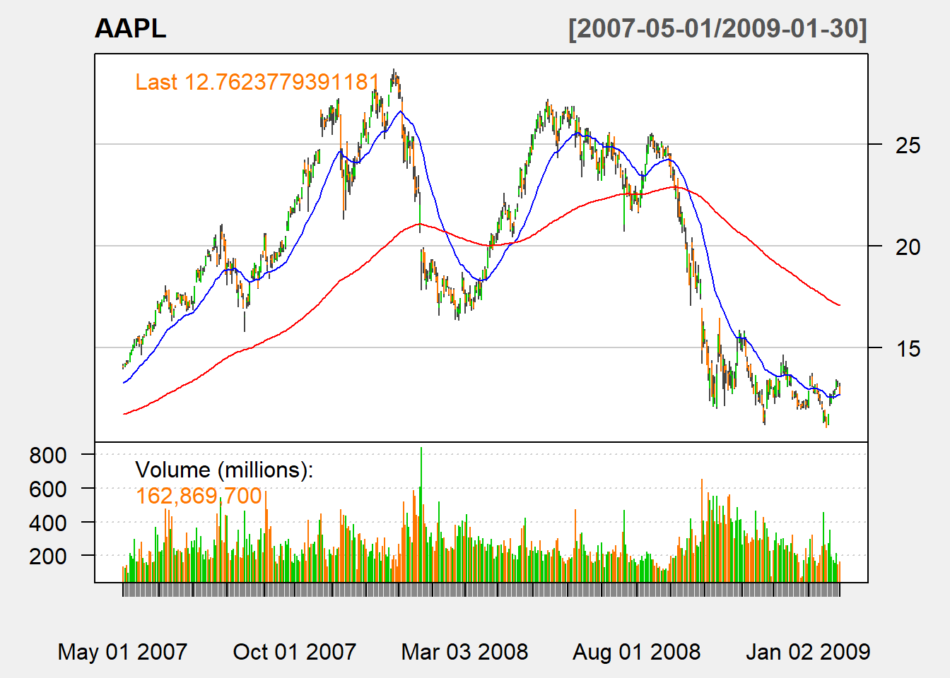
5.3.3 Charting

chartSeries(AAPL,
            subset='2007-05::2009-01',
            theme=chartTheme('white'))
addEMA(n=30,on=1,col = "blue")
addEMA(n=200,on=1,col = "red")