8.2 Blotter Package
Since working through quanstrat package requires the blotter package, which is rather complicated, we demostrate first how the blotter pacakge works first.
As we have seen, recording tranasction of stocks, keeping track of cash and stock holding, and evaluate return is rather messy. The blotter package is mainly for this purpose.
We first need to setup the working space.
We need to setup the currency and declare the data is the stock (using FinancialInstrument package).
The multipler is always one for stock, and currency is USD for US stock.
options("getSymbols.warning4.0"=FALSE)
from ="2008-01-01"
to ="2012-12-31"
symbols = c("IBM")
currency("USD")
getSymbols(symbols, from=from, to=to,
           adjust=TRUE)
stock(symbols, currency="USD", multiplier=1)
initEq=10^6
To start, we initialize account and portfolio where:
Porfolio: stores which stocks to be traded
Account: stores which money transactions
.blotter <-new.env()
rm("account.buyHold",pos=.blotter)
rm("portfolio.buyHold",pos=.blotter)

initPortf("buyHold", symbol=symbols)
initAcct("buyHold", portfolios = "buyHold",
         initEq = initEq)
8.2.1 Buy and hold
To illustrate, we just consider buy and hold strategy on IBM:
- Buy on the first day at closing price
- Sell on the last day at closing price
We first get the price and timing data:
Buy.Date <- first(time(IBM))
Buy.Price <- as.numeric(Cl(IBM[Buy.Date,]))
Sell.Date <- last(time(IBM))
Sell.Price <- as.numeric(Cl(IBM[Sell.Date,]))
Qty <- initEq/Buy.Price
We first add buy transactions to the system using the function addTxn:
addTxn(Portfolio = "buyHold",
       Symbol = "IBM",
       TxnDate = Buy.Date,
       TxnQty = Qty,
       TxnPrice = Buy.Price,
       TxnFees = 0)
Then we add the sell transactions:
addTxn(Portfolio = "buyHold",
       Symbol = "IBM",
       TxnDate = Sell.Date,
       TxnQty = -Qty,
       TxnPrice = Sell.Price,
       TxnFees = 0)
Now we can update the account based on the added transactions:
updatePortf(Portfolio = "buyHold")## [1] "buyHold"updateAcct(name = "buyHold")## [1] "buyHold"updateEndEq(Account = "buyHold")## [1] "buyHold"We can chart our trading positions:
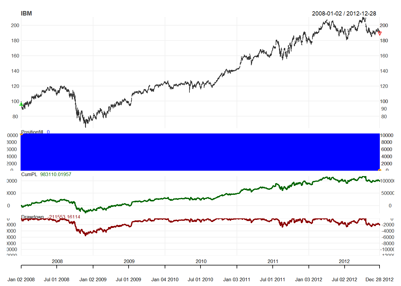
chart.Posn("buyHold", Symbol = "IBM")
We can see the trading statistics
out <- perTradeStats("buyHold", "IBM")
t(out)
## [,1]
## Start "2008-01-02 08:00:00"
## End "2012-12-28 08:00:00"
## Init.Qty "10446.77"
## Init.Pos "10446.77"
## Max.Pos "10446.77"
## End.Pos "0"
## Closing.Txn.Qty "-10446.77"
## Num.Txns "2"
## Max.Notional.Cost "1e+06"
## Net.Trading.PL "983110"
## MAE "-302740.5"
## MFE "1194663"
## Pct.Net.Trading.PL "0.98311"
## Pct.MAE "-0.3027405"
## Pct.MFE "1.194663"
## tick.Net.Trading.PL "9410.662"
## tick.MAE "-30274048"
## tick.MFE "119466318"
## duration "157420800 secs"8.2.2 Buy Filter Rule
We use blotter package to apply simple filter rule
buy 1000 units signal if buy signal
hold otherwise
We first Download Data:
from ="2011-10-01"
to ="2012-12-31"
symbols = c("MSFT")
currency("USD")
getSymbols(symbols, from=from, to=to,
           adjust=TRUE)
stock(symbols, currency="USD", multiplier=1)
initEq=10^6
Then setup the account and portfolio:
.blotter <-new.env()
rm("account.filter",pos=.blotter)
rm("portfolio.filter",pos=.blotter)

initPortf("filter", symbol=symbols)
initAcct("filter", portfolios = "filter",
         initEq = initEq)
Here we generate trading indicator:
price <- Cl(MSFT)
r <- price/Lag(price) - 1
delta<-0.03
signal <-c(NA)
for (i in 2: length(price)){
    if (r[i] > delta){
         signal[i]<- 1
    } else if (r[i]< -delta){
         signal[i]<- -1
    } else
         signal[i]<- 0
}
signal<-reclass(signal,Cl(MSFT))
This convert trading indicator to trading signal:
trade <- Lag(signal)
trade <- na.fill(trade,0)
Now we are ready to apply trading signal into trading action:
for (i in 1:length(price)){
  if (as.numeric(trade[i]) == 1){
    addTxn(Portfolio = "filter",
           Symbol = "MSFT",
           TxnDate = time(price[i]),
           TxnQty = 1000,
           TxnPrice = price[i],
           TxnFees = 0)
  }
    if (as.numeric(trade[i]) == -1){
    addTxn(Portfolio = "filter",
           Symbol = "MSFT",
           TxnDate = time(price[i]),
           TxnQty = -1000,
           TxnPrice = price[i],
           TxnFees = 0)
  }
}
We now update the account and do charting:
updatePortf(Portfolio = "filter")
updateAcct(name = "filter")
updateEndEq(Account = "filter")
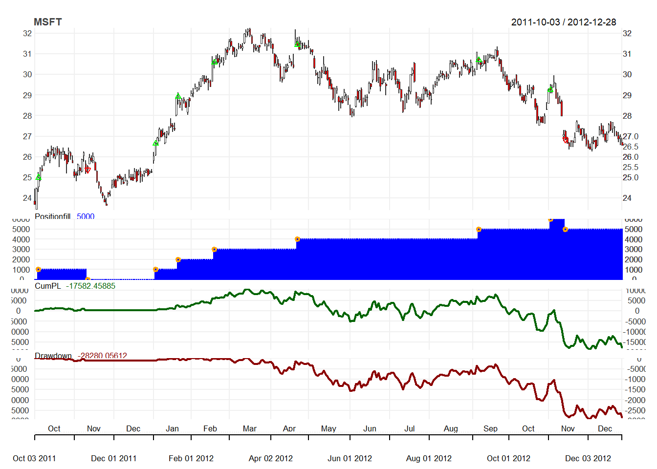
chart.Posn("filter", Symbol = "MSFT")
Finally, we check the trading statistics:
out <- perTradeStats("filter", "MSFT")
t(out)
## [,1] [,2]
## Start "2011-10-05 08:00:00" "2012-01-04 08:00:00"
## End "2011-11-10 08:00:00" "2012-12-28 08:00:00"
## Init.Qty "1000" "1000"
## Init.Pos "1000" "1000"
## Max.Pos "1000" "6000"
## End.Pos " 0" "5000"
## Closing.Txn.Qty "-1000" "-5000"
## Num.Txns "2" "7"
## Max.Notional.Cost " 24989.77" "177548.89"
## Net.Trading.PL " 376.4411" "-17958.8999"
## MAE " 0.00" "-18858.89"
## MFE " 1370.625" "10321.156"
## Pct.Net.Trading.PL " 0.01506381" "-0.10114904"
## Pct.MAE " 0.000000" "-0.106218"
## Pct.MFE "0.05484743" "0.05813135"
## tick.Net.Trading.PL " 37.64411" "-299.31500"
## tick.MAE " 0" "-1885889"
## tick.MFE " 137062.5" "1032115.6"
## duration " 3110400 secs" "31017600 secs"