5.4 Bollinger band

A channel (or band) is an area that surrounds a trend within which price movement does not indicate formation of a new trend.

For Bollinger band, channel is drawn over a trend line plus/minus 2 SD:

Trend line: SMA or EMA of price (price can be closing price or average of high, low, and close)

Bandwidth: determined by the asset volatility \[B_t(n)=k\times stdev(P_t, n)\] where usually we have \(k=2\) and \(n=20\).

The lower and upper bands are \[up_t = P_t + B_t(n) \text{, and } down_t=P_t - B_t(n).\]

To denote the location of the price, we use \[\%B=\frac{P_t-down_t}{up_t-down_t}\]

where it is greater 1 if it is above the upper band, and less than 0 when it is below the lower band.

myBBands <- function (price,n,sd){
  mavg <- SMA(price,n)
  sdev <- rep(0,n)
  N <- nrow(price)
  for (i in (n+1):N){
    sdev[i]<- sd(price[(i-n+1):i])
  }
  up <- mavg + sd*sdev
  dn <- mavg - sd*sdev
  pctB <- (price - dn)/(up - dn)
  output <- cbind(dn, mavg, up, pctB)
  colnames(output) <- c("dn", "mavg", "up", 
        "pctB")
  return(output)
}

Now let us put our code to work:

bb <-myBBands(Cl(AAPL),n=20,sd=2)
tail(bb,n=5)

##                  dn     mavg       up      pctB
## 2012-12-21 70.37089 78.45000 86.52911 0.2363574
## 2012-12-24 70.15448 77.95457 85.75466 0.2663762
## 2012-12-26 69.84213 77.44186 85.04158 0.2265597
## 2012-12-27 69.69496 76.95700 84.21904 0.2674898
## 2012-12-28 69.75519 76.38721 83.01924 0.2294459

5.4.1 TTR

We use BBands in TTR to calculate:

bb <-BBands(Cl(AAPL),n=20, sd=2)
tail(bb,n=5)

##                  dn     mavg       up      pctB
## 2012-12-21 70.57545 78.45000 86.32455 0.2295084
## 2012-12-24 70.35199 77.95457 85.55716 0.2603070
## 2012-12-26 70.03456 77.44186 84.84915 0.2194561
## 2012-12-27 69.87884 76.95700 84.03516 0.2614495
## 2012-12-28 69.92311 76.38721 82.85132 0.2224173

Note that it is different from above. It turns out that the standard deviation used is population instead of sample one. We only need to correct it by the factor of \(\sqrt{(n-1)/n}\).

myBBands <- function (price,n,sd){
  mavg <- SMA(price,n)
  sdev <- rep(0,n)
  N <- nrow(price)
  for (i in (n+1):N){
    sdev[i]<- sd(price[(i-n+1):i])
  }
  sdev <- sqrt((n-1)/n)*sdev
  up <- mavg + sd*sdev
  dn <- mavg - sd*sdev
  pctB <- (price - dn)/(up - dn)
  output <- cbind(dn, mavg, up, pctB)
  colnames(output) <- c("dn", "mavg", "up", 
        "pctB")
  return(output)
}

Now we can reoncile the two:

bb <-myBBands(Cl(AAPL),n=20,sd=2)
tail(bb,n=5)

##                  dn     mavg       up      pctB
## 2012-12-21 70.57545 78.45000 86.32455 0.2295084
## 2012-12-24 70.35199 77.95457 85.55716 0.2603070
## 2012-12-26 70.03456 77.44186 84.84915 0.2194561
## 2012-12-27 69.87884 76.95700 84.03516 0.2614495
## 2012-12-28 69.92311 76.38721 82.85132 0.2224173

5.4.2 Trading Signal

Buy signal arises when price is above the band.

Sell signal arises when price is above the band.

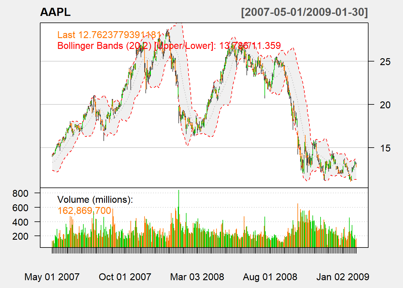
5.4.3 Charting

chartSeries(AAPL,
            subset='2007-05::2009-01',
            theme=chartTheme('white'))
addBBands(n=20,sd=2)