1.3 Process of Doing Data Science
Understand what data science is about is just a start of becoming a data scientist. Once the goal is set. The next task is to select a correct path and work hard to to reach your destination. The path is important which can be shorter or longer, or direct and smooth, or curvy and bumpy. It is vital to follow a short and smooth path. This path is the data science project process. Figure 1.3 is the 6 steps process, which is inspired by the CRISP (Cross Industry Standard Process for Data Mining) (Pete Chapman and Wirth 2000), (Shearer 2000) and KDD (knowledge discovery in data bases) process (Li 2018).
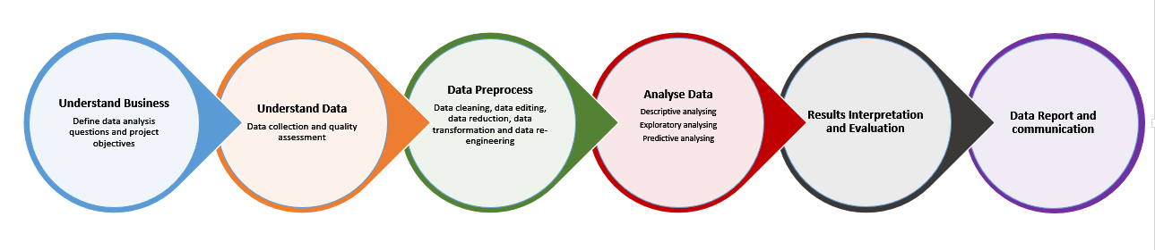
Figure 1.3: Process of doing Data Science
Step 1: Understand the Problem - Define Objectives
Any data analysis must begin with business issues. With business issues a number of questions should be asked. These questions have to be the right questions and measurable, clear and concise. Define analysis question is regarded as define a Data Requirements engineering and to get a a data project specification. It starts from a business issue and asking relevant questions, only after you fully understand the problem and the issues you may be able to turn practical problem into analytical questions.
For example, start with a business issue: A contractor is experiencing rising costs and is no longer able to submit competitive contract proposals. One of many questions to solve this business problem might include: Can the company reduce its staff without compromising quality? Or, can company find alternative suppler on the production chain?
Once you have questions, you can start to thinking about data required for analysis. The data required for analysis is based on questions. The data necessary as inputs to the analysis can then be identified (e.g., Staff skills and performance). Specific variables regarding a staff member (e.g., Age and Income) may be specified and obtained. Data type can be defined as numerical or categorical.
After you defined you analytical questions. It is important to Set Clear evaluation of your project to measurement how success of your project.
This generally breaks down into two sub-steps: A) Decide what to measure, and B) Decide how to measure it.
A) What To Measure?
Using the contractor example, consider what kind of data you’d need to answer your key question. In this case, you would need to know the number and cost of current staff and the percentage of time they spend on necessary business functions. This is what is called in business as KPI - Key performance indicators. In answering this question, you likely need to answer many sub-questions (e.g., Are staff currently under-utilized? If so, what process improvements would help?). Finally, in your decision on what to measure, be sure to include any reasonable objections any stakeholders might have (e.g., If staff are reduced, how would the company respond to surges in demand?).
B) How To Measure?
Thinking about how you measure the success fo your data science project, the deep end is to measure some key performance indicators. They are the data you have chosen to use in the previous step. So measure your data is just as important, especially before the data collection phase, because your measuring process either backs up or discredits your project later on. Key questions to ask for this step include:
- What is your time frame? (e.g., annual versus quarterly costs)
- What is your unit of measure? (e.g., USD versus Euro)
- What factors should be included? (e.g., just annual salary versus annual salary plus cost of staff benefits)
Step 2: Undertand Data - Knowing your Raw Materials
The second step is understand data. It includes Data collection and Data Validation. With problem understood and analytical questions defined and your validation criteria and measurements set, It is time to collect data.
Data Collection
Before collect data, the data source has to be determined based on the relevance. Variety of data source may be assessed and accessed to get relevant data. These data source may include an existing databases, or organization’s file system, or a third party service or even open web sources. They could provide redundant, or complementary, sometimes conflict data. it has to be cautious to select right data source from the very beginning. sometimes you need gather data via observation or interviews, then develop an interview template ahead of time to ensure consistency. it is a good idea to Keep your collected data organized in a log with collection dates and add any source notes as you go (including any data normalization performed). This practice validates your data and any conclusions down the road.
Data Collection is the actual process of gathering data on targeted variables identified as data requirements. The emphasis is on ensuring correct and accurate data collection, which means correct procedure was taken and appropriate measurements were adopted. the maximum efforts were spent to ensure the data quality. Remember that data Collection provides both a baseline to measure and a target to improve for a successful data science project.
Data Validation
Data validation id the process to Assess data quality. It is to ensure the collected data have reached quality requirements identified in the step 1, that is, they are useful and correct. The usefulness is the most important aspect. Regardless how accurate your data collections can be, if it is not useful, anything follows are just waste. It is hard to define the usefulness. depends on the problem at hand and the requirements for the find al delivery. The usefulness can various from a strong correlation between the raw data and the expected outcomes, to direct prediction power from the raw data to the concequence variables. Gernrally data validation can include:
- Data type validation
- Range and constraint validation
- Code and cross-reference validation
- Structured validation
- Consistency validation
- Relevancy validation
Step 3: Data Preprocess - Get your Data Ready
Data preprocess is step that takes data processing method and technique to transforms raw data into a formatted and understandable form and ready for analyzing. Real world data is often incomplete, inconsistent, and is likely to contain many errors. Data preprocess is a proven method of resolving such issues. Tasks of data preprocess may include:
Data cleaning. The process of detecting and correcting (or removing) corrupt or inaccurate records from a record set, table, or database. It normally includes identifying incomplete, incorrect, inaccurate or irrelevant data and then replacing, modifying, or deleting the dirty or coarse data. After cleansing, a data set should be consistent with other data sets.
Data editing. The process involves changing and adjusting of collected data. The purpose is to ensure the quality of the collected data. Data editing should be done by fully understand the data collected and the data requirement specification. Editing data without them can be disastrous.
Data reduction. The process and methods used to reduce data quantity to fit for analyzing. Raw data set collected or selected for analysis can be huge, then it could drastically slow down the analysis process. Reducing the size of the data set without jeopardizing the data analysis results is often desired. It includes records’ number reduction and data attributes reduction. Methods used for reduce data records size includes Sampling and Modelings (e.g., regression or log-linear models or histograms, clusters, etc). Methods used for attributes reduction include Feature selection and Dimension reduction. Feature selection means removal of irrelevant and redundant features. such operation should not lose information the data set has. Data analysis algorithms work better if the dimensionality, which is the number of attributes in a data object is low. Data compression techniques (e.g., wavelet transforms and principal components analysis), attribute subset selection (e.g., removing irrelevant attributes as discussed in previous paragraph), and attribute construction (e.g., where a small set of more useful attributes is derived from the large numbers of attributes in the original data set) are useful techniques.
Data transformation sometimes referred to as data munging or data wrangling. It is the process of transforming and mapping data from one data form into another format with the intent of making it more appropriate and valuable for downstream analytics. It is often that data analysis method requires data to be analyzed have certain format or possesses certain attributes. For example, classification algorithms require that the data be in the form of categorical (nominal) attributes; algorithms that find association patterns require that the data be in the form of binary attributes. Thus, it is often necessary to transform a continuous attribute into a categorical attribute, which is called Discretization, and both continuous and discrete attributes may need to be transformed into one or more binary attributes, whci iscalled Banalization. Other methods include Scaling and normalization.Scaling changes the bounds of the data, and can be useful, for example, when you are working with data in different units. Normalization scales data sets to a smaller range such as [0.0, 1.0].
Data re-engineering Re-engineering data is necessary when raw data come from many different data sources and in different format. Data re-engineering similar with data transformation can be done in both record level and in attributes level. Record level re-engineering is also called data Integration, which integrates variety of data into one file or place and in one format for analysis. for predictive analysis with a model, data re-enginering is also including split a given data set into two subsets called “Training” and “Test” Set.
Step 4: Data Analyese - Building Models
After your collected data being preprocessed and suitable for analysis. Now you can drill down and attempt to answer your question from Step 1 with the actions called Data Analyzing. It is the core activity in data science project process by writing, executing, and refining computer programs that utilize some analytical methods and algorithms to obtain insights from data sets. There are three broad categories of data analytical methods: Descriptive data analysis (DDA), Exploratory data analysis (EDA) and Predictive data analysis (PDA). DDA and EDA uses quantitative and statistical methods on data sets and data attributes measurements and their value distributions while DDA focus on numeric summary and EDA emphasis on graphical (plot) means, PDA involves model building and machine learning. In a data science project, data analyzing is generally starting from Descriptive analysis, and goes further with Exploratory analysis, and finally end up with a tested and optimized prediction model for predicting. However, it does not necessarily mean that the methods use in a data analysis project have to stick on this order. As matte of fact, the most project involves a recursive process and a mixture of all the three methods. For example, An exploratory analysis can be utilized in a feature engineering step to prepare a predictor of a prediction model, which is used to predict some missing values of a particular attribute in a given dataset for accurate describe the attribute value distribution.
Descriptive data analysis
It is the simplest type of analysis. It describes and summarizes a data set quantitatively. Descriptive analysis generally starts with an univariate analysis, meaning describing a single variable (can also be called attribute, column or field) of the data. The appropriate depends on the level of measurement. For nominal variables, a frequency table and a listing of the modes are sufficient. For ordinal variables the median can be calculated as a measure of central tendency and the range (and variations of it) as a measure of dispersion. For interval level variables, the arithmetic mean (average) and standard deviation are added to the toolbox and, for ratio level variables, we could add the geometric mean and harmonic mean as measures of central tendency and the coefficient of variation as a measure of dispersion. However, there are many other possible statistics which covers areas such as location (“middle” of the data), dispersion (range or spread of data) and shape of the distribution. Moving up to two variables, descriptive analysis can involve measures of association such as computing a correlation coefficient or covariance. Descriptive analysis’ goal is to describe the key features of the sample numerically. It should shed light on the key numbers that summarize distributions within the data, may describe or show the relationships among variables with metrics that describe association, or by tables that cross tabulation counts. Descriptive analysis is typically the first step on the data analysis ladder, which only tries to get a sense of the data.
Explorative data analysis
Descriptive analysis is very important. However, numerical summaries can only get you so far. One problem is that it can only converting a large number of values down to a few summary numbers. Unsurprisingly, different samples with different distributions, shapes, and properties can result in the same summary statistics. This will cause problems. When you are looking a simple single summary statistic, the mean of a single variable, there can be a lot of possible “solutions” or samples. The typical example is Anscombe’s quartet (Anscombe 1973), it comprises four datasets that have nearly identical simple statistical properties, yet appear very different when graphed. Most kinds of statistical calculations rest on assumptions about the behavior of the data. Those assumptions may be false, and then the calculations may be misleading. We ought always to try and check whether the assumptions are reasonably correct; and if they are wrong we ought to be able to perceive in what ways they are wrong. Graphs are very valuable for these purposes.
EDA allows us to challenge or confirm our assumptions about the data. It is a good tool to be used in data prerpocess. We often have pretty good expectations of what unclean data might look like, such as outliers, missing data, and other anomalies, perhaps more so than our expectations of what clean data might look like. With the more we understood data, we could develop our intuition of what factors and possible relations at are play. EDA, with its broad suite of ways to view the data points and relationships, provides us a range of lenses with which to study story that data is telling us. That in turn, helps us to come up with new hypotheses of what might be happening. Further, if we understood which variables we can control, which levers we have to work within a system to drive the metrics such as business revenue or customer conversion in the desired direction. EDA can also highlight gaps in our knowledge and which experiments might make sense to run to fill in those gaps.
The basic tools of EDA are plots, graphs and summary statistics. Generally speaking, it’s a method of systematically going through the data, plotting distributions of all variables (using box plots), plotting time series of data, transforming variables, looking at all pairwise relationships between variables using scatterplot matrices, and generating summary statistics for all of them or identifying outliers.
Predictive data analysis
Predictive analysis builds upon inferential analysis, which is to learn about relationships among variables from an existing training data set and develop a model that can predict values of attributes for new, incomplete, or future data points. Inferential analysis is a type of analysis that from a dataset sample in hand infer some information, which might be parameters, distributions, or relationships about the broader population from which the sample came. We typically infer metrics about the population from a sample because data collection is too expensive, impractical, or even impossible to obtain all data. The typical process of inferential analysis includes testing hypothesis and deriving estimates. There are a whole slew of approaches and tools in predictive analysis. Regression is the broadest family of tools. Within that, however, are a number of variants (lasso, ridge, robust etc.) to deal with different characteristics of the data. Of particular interest and power is Logistic Regression that can be used to predict classes. For instance, spam/not spam used to be mostly predicted with a Naïve Bayes predictor but nowadays logistic regression is more common. Other techniques and what come under the term Machine Learning include neural networks, tree-based approaches such as classification and regression trees, random forests, support vector machines (SVM), and k-nearest neighbours.
Step 5: Results Interpretation and Evaluation
After analyzing your data and get some answers about your original questions, it is possible that you need conduct further research and more analysis. Let us suppose that you are happy with the analysis results you have. It is finally time to interpret your results. As you interpret your analysis, keep in mind that you cannot ever prove a hypothesis true: rather, you can only fail to reject the hypothesis. Meaning that no matter how much data you collect, chance could always interfere with your results. Interpreting the results of analysis, you should thinking of how close the results address the original problems by asking yourself these key questions:
- Does the data answer your original question? How?
- Does the data help you defend against any objections? How?
- Are there any limitation on your conclusions, any angles you haven’t considered?
If your interpretation of the data holds up under all of these questions and considerations, then you likely have come to a productive conclusion. However, there could be a chance that you may find you might need to revise your original question or collect more data and you may need to roll the ball from the starting line. Again. Either way, this initial analysis of trends, correlations, variations and outliers are not completely wasted. They help you focus your data analysis on better answering your question and any objections others might have. That is the next step report and communication.
Step 6: Data Report and Communication
Whereas the analysis phase involves programming and run programs on different computer platforms, the reporting involves narrative the results of analysis, thinking how close the results address the original problems and communicating about the outputs of analyses with interesting parties in many cases in visual formats. During this step, data analysis tools and software are helpful but visual tools are intuitive and worth a lot of words. Visio, tableau (https://www.tableau.com/), Minitab (https://www.minitab.com/) and Stata (https://www.stata.com/) are all good software packages for advanced statistical data analysis. There are also plenty of open source data visualization tools available.
It is important to note that the above 6 steps process is not a linear process. Any discovery of useful relationships and valuable patterns are enabled by a set of iterative activities. Iteration can occur in a single step or in a few steps in any point in the process.
References
Anscombe, F. J. 1973. “Graphs in Statistical Analysis.” American Statistician 27 (1). https://en.wikipedia.org/wiki/Anscombe%27s_quartet.
Li, Gagnmin. 2018. Fundation of Big Data Analytics: Concepts, Technologies, Methods and Business. 1st ed. Beijing, China: Science press.
Pete Chapman, Randy Kerber, Julian Clinton, and Rudiger Wirth. 2000. CRISP-Dm 1.0 Step-by-Step Data Mining Guides. https://www.the-modeling-agency.com/crisp-dm.pdf.
Shearer, C. 2000. “The Crisp-Dm Model: The New Blueprint for Data Mining.” Data Warehousing 5: 13–22.