12.3 Model Interpretation
There are a number of ways to interpret a model. The commonly used methods are explaining model’s performance and its predictors’ importance.
Model’s Performance Measure
There are many different metrics that can be used to evaluate a prediction model. Depends on the type of the model, the different metrics are used to measure its performance. Random forest models built with the Caret package from R, the default metrics are Accuracy and Kappa. We have seen them in Chapters 9, 10, and Chapter 11.
Accuracy is the percentage of correctly classified instances out of all instances. It is useful on binary classification problems because it can be clear on exactly how the accuracy breaks down across the classes through a confusion matrix.
Kappa is also called Cohen’s Kappa. It is a normalized accuracy measurement. The normalization is at the baseline of random chance on the dataset. It is a more useful measure to use on problems that have an imbalance in the classes (e.g. 70-30 split for classes 0 and 1 and you can achieve 70% accuracy by predicting all instances are for class 0).
For example, our best random forest model was RF_model2. We can use these metrics to briefly explain our model’s performance. Let us load model RF_model2 and print out its model details:
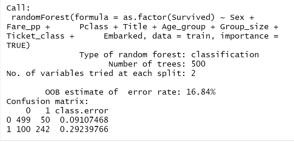
Figure 12.1: The detials of RF_model2
We can see that the model’s estimated accuracy (by the model construction) is 83.16%. That is 1-OOB. Notice that the default parameters of the model are: mtry = 2 and ntree = 500.
Looking into the model’s confusion matrix, the RF_model2’s overall prediction errors can be interpreted based on the two classes “survived” or “perished”: error on the predicted perished is 9.28% and error on the predicted survive is 28.07%. It is important to know the differences between them, as in many applications, they reflect the “positive error” and the “negative error”. Depending on the interest, one class is regarded as the positive, the other will be the negative class. However, our model’s performance is better on perished than on survived.
We can drill down a bit more, for example, we can check the top 10 decision trees’ accuracy (error rate) among the 500 randomly generated trees by the RF model, and we can also check the average error rate among the 500 trees.
##             OOB          0         1
##  [1,] 0.2192192 0.16176471 0.3100775
##  [2,] 0.1963964 0.13157895 0.3004695
##  [3,] 0.1953010 0.12351544 0.3115385
##  [4,] 0.2110092 0.13404255 0.3344710
##  [5,] 0.2009804 0.11729622 0.3354633
##  [6,] 0.2028640 0.13203883 0.3157895
##  [7,] 0.1953216 0.12571429 0.3060606
##  [8,] 0.1900922 0.11588785 0.3093093
##  [9,] 0.1881414 0.11090573 0.3125000
## [10,] 0.1755379 0.09392265 0.3058824
## OOB 0 1
## Min. :0.1582 Min. :0.08379 Min. :0.2544
## 1st Qu.:0.1650 1st Qu.:0.08925 1st Qu.:0.2807
## Median :0.1661 Median :0.09107 Median :0.2865
## Mean :0.1670 Mean :0.09298 Mean :0.2858
## 3rd Qu.:0.1684 3rd Qu.:0.09654 3rd Qu.:0.2895
## Max. :0.2192 Max. :0.16176 Max. :0.3355To verify the constructed model’s prediction accuracy, We did cross validations on the model RF_model2 and produced a CV model RF_model2_cv, We can show the results too.
## Random Forest
##
## 712 samples
##   8 predictor
##   2 classes: '0', '1'
##
## No pre-processing
## Resampling: Cross-Validated (10 fold, repeated 5 times)
## Summary of sample sizes: 641, 640, 642, 641, 640, 641, ...
## Resampling results across tuning parameters:
##
##   mtry  Accuracy   Kappa
##    2    0.8105369  0.5725714
##   17    0.8404408  0.6518406
##   32    0.8312040  0.6320845
##
## Accuracy was used to select the optimal model using the largest value.
## The final value used for the model was mtry = 17.
The CV model confirmed the RF model’s best accuracy is 84.04% and the kappa is 65.18%. But it revealed that the model has an overfitting problem. We, therefore, fine-tuned the RF model (with the different predictors that were identified by the fine tune itself). The fine-tuned model’s accuracy is also around 84%.
Visualise Model’s Prediction
We have said that a graph is worth hundreds of words. Visualising analytical results is important and useful. But directly visualise a model’s prediction is difficult since the RF model has over 3 dimensions. Humans are not good at understanding any visual objects that have more than 3 dimensions even there are ways of visualization. So we need to find a way of reducing a model’s dimension. Rtsne package from R is exactly designed for this purpose. You can check Rtsne document to find more details. Basically, Function Rtsne converts a multiple dimension dataframe’s values into a 2D-coordinates. We can then use these 2d-coordinates to plot our response variable’s value on it.

Figure 12.2: 2D Visualization of Model RE_model2’s Prediciton
The above code filtered the train dataset with only predictors used in RF_model2 through the features variable. It calls function Rtsne to generate two-dimension coordinates for each data sample in train based on the values of the attributes specified by features. The coordinates are stored in the sub-array Y. So we can dot plot the value of survived on the coordinates. Figure 12.2 shows the two-class distributions based on the features’ values, which were used as predictors in the RF_model2.
Importance of the Model’s Predictors
Another element of a model, which is worthwhile to report, is the predictors’ importance. In our best random forest model RF_model2, The predictors’ importance is shown in Figure 12.3.

Figure 12.3: The ordered importance of the predictors
##          Sex        Title      Fare_pp       Pclass Ticket_class   Group_size
##  0.101687822  0.087587574  0.040794545  0.038645459  0.028333273  0.027816253
##    Age_group     Embarked
##  0.016016542  0.006786278
From Figure 12.3, we can see that the MeanDecreaseAccu and the MeanDecreaseGini measure provide a different order. The difference reflects the different evaluation metrics. Briefly,
Mean Decrease in Impurity (MDI), the metrics is
GINIindex, it can be biased towards categorical features which contain many categories.Mean Decrease in Accuracy (MDA), the metrics is accuracy, it can provide low importance to other correlated features if one of them is given high importance.
If a model’s performance report sets up the tasks for further analysis, then the predictors’ importance report can set up the attributes to which features re-engineering should start with.