8.1 Decision Tree in Hunt’s Algorithm
Hunt’s algorithm builds a decision tree in a recursive fashion by partitioning the training dataset into successively purer subsets. Hunt’s algorithm takes three input values:
- A training dataset, \(D\) with a number of attributes,
- A subset of attributes \(Att_{list}\) and its testing criterion together to form a
'test condition', such as'age>=25'is a test condition, where,'age'is the attribute and'>=25'is the test criterion. - A
Attribute_selection_method, it refers a procedure to determine the best splitting.
The general recursive procedure is defined as below (Pang-Ning Tan 2005):
- Create a node \(N\), suppose the training dataset when reach to note \(N\) is \(D_{N}\). Initially, \(D_{N}\) is the entire training set \(D\). Do the following:
- If \(D_{t}\) contains records that belong the same class \(y_{t}\), then \(t\) is a leaf node labelled as \(y_{t}\);
- If \(D_{t}\) is not an empty set but \(Att_{list}\) is empty, (there is no more test attributes left untested), then \(t\) is a leaf node labelled by the label of the majority records in the dataset;
- If \(D_{t}\) contains records that belong to more than one class and \(Att_{list}\) is not empty, use
Attribute_selection_methodto choose next best attribute from the \(Att_{list}\) and remove that list from \(Att_{list}\). use the attribute and its condition as next test condition. - Repeat steps 2,3 and 4 until all the records in the subset belong to the same class.
There are two fundamental problems that need to be sorted before Hunt’s algorithm can work:
- How to form a ‘test condition’? particularly when non-binary attributes exist?
- How to define the ‘best test conditions’, so very loop the best test condition can be used in a decision tree?
How to Form a Test Condition?
Decision tree algorithms must provide a method for expressing a test condition and its corresponding outcomes for different attribute types.
- Binary Attributes. The test condition for a binary attribute is simple because it only generates two potential outcomes, as shown in figure 8.2.
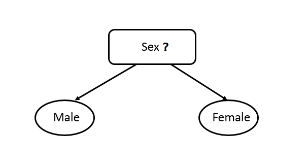
Figure 8.2: Test condition for binary attributes.
- No-binary attributes. No-binary attributes depend on the types of nominal or ordinal, it can have different ways of the split. A nominal attribute can have many values, its test condition can be expressed in two ways, as shown in Figure 8.3. For a multiway split, see Figure 8.3(a), the number of outcomes depends on the number of distinct values for the corresponding attribute. For example, if an attribute such as age has three distinct values: youth, m_aged, or senior. Its test condition will produce a three-way split or a binary split. Figure 8.3(b) illustrates three different ways of grouping the attribute values for age into two subsets.
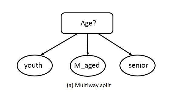
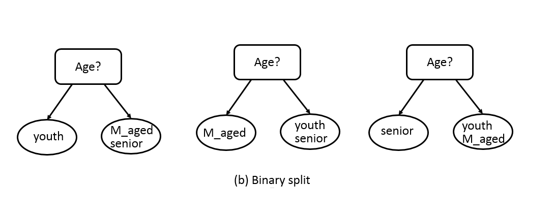
Figure 8.3: Test condition for no-binary attributes.
- Continuous Attributes. For continuous attributes, the test condition can be constructed as a comparison test \((A<v)\) or \((A≥v)\) with binary outcomes, or a range query with outcomes of the form \(v_i≤A<v_{i+1}\), For \(i=1,…,k\). The difference between these approaches is shown in Figure 8.4. For the binary case, the decision tree algorithm must consider all possible split positions v, and it selects the one that produces the best partition. For the multiway split, the algorithm must consider all possible ranges of continuous values.
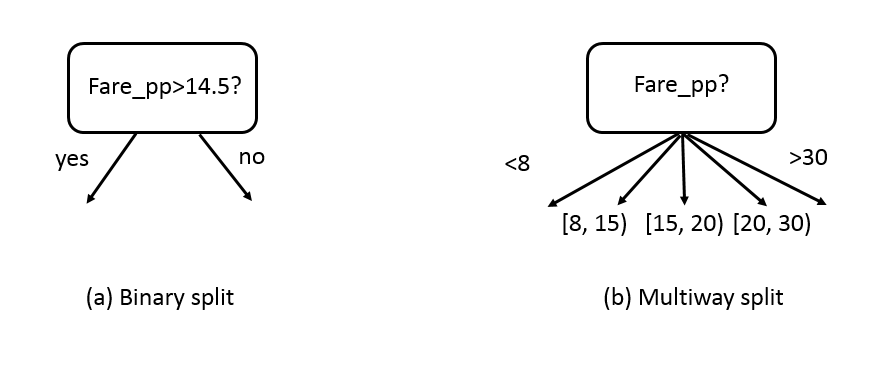
Figure 8.4: Test condition for continuous attributes.
How to Determine the Best Split Condition?
The method used to define the best split makes different decision tree algorithms. There are many measures that can be used to determine the best way to split the records. These measures are defined in terms of the class distribution of the records before and after splitting. The best splitting is the one that has more purity after the splitting. If we were to split \(D\) into smaller partitions according to the outcomes of the splitting criterion, ideally each partition after splitting would be pure (i.e., all the records that fall into a given partition would belong to the same class). Instead of defining a split’s purity, the impurity of its child node is used. There are a number of commonly used impurity measurements: Entropy, Gini Index and Classification Error.
Entropy: measures the degree of uncertainty, impurity, or disorder. The formula for calculate entropy is as shown below:
\[\begin{equation} E(x)= ∑_{i=1}^{n}p_ilog_2(p_i), \tag{8.1} \end{equation}\]
Where \(p\) represents the probability and \(E(x)\) represents the entropy.
Gini Index: also called Gini impurity, measures the degree of probability of a particular variable being incorrectly classified when it is chosen randomly. The degree of the Gini index varies between zero and one, where zero denotes that all elements belong to a certain class or only one class exists, and one denotes that the elements are randomly distributed across various classes. A Gini index of 0.5 denotes equally distributed elements into some classes.
The formula used to calculate Gini index is shown below:
\[\begin{equation} GINI(x) = 1- ∑_{i=1}^{n}p_i^2, \tag{8.2} \end{equation}\]
Where \(p_i\) is the probability of an object being classified to a particular class.
Classification Error measures the misclassified class labels. It is calculated with the formula shows below: \[\begin{equation} Classification error(x)= 1 - max_{i}p_i. \tag{8.3} \end{equation}\]
Among these three impurity measurements, Gini is Used by the CART (classification and regression tree) algorithm for classification trees, and Entropy is Used by the ID3, C4.5, and C5.0 tree-generation algorithms.
With the above explanation, we can now say that the aims of a decision tree algorithm are to reduce the Entropy level from the root to the leaves and the best tree is the one that takes order from the most to the least in reducing the Entropy level.
The good news is that we do not need to calculate the impurity of each test condition to build a decision tree manually. Most tools have the tree construction built-in already. We will use the R package called rpart to build decision trees for our Titanic prediction problem.
References
Pang-Ning Tan, Vipin Kumar, Michael Steinbach. 2005. Introduction to Data Mining. 1st ed. Addison Wesley.