6.2 Process of Predcitive Data Analysis
The process of predictive data analysis is called predictive modelling. It is generally involves three steps:
- Predictor selection,
- model construction, and
- model evaluation.
Predictor Selection
A predictor, in data science, is an attribute that a prediction model used to predict values of another attribute. The attribute to be predicted is called consequencer (or dependent, or response, we may use them exchangeable). Generally, a data object can have a large number of attributes, which can potentially be used as predictors by a model to produce consequencer. Most models do not use all of the data attributes, instead only a number of selected attributes are used.
The selection is based on the relationship between the predictor and the consequencer and also the relationship among the predictors. Filter and wrapper are the most common methods used in the attributes selection:
Filters. The filter is a method that examines each predictor in turn. A numerical measure is calculated, representing the strength of the correlation2 between the predictor attribute and the consequencer. This correlation is conventionally called the prediction power of a predictor in the prediction modelling. The only predictor attributes where the correlation measure3 exceeds a given threshold are selected or simply select the fixed number of the top attributes which has higher correlation measure.
Wrappers. A wrapper takes a group of predictors and considers the “value add” of each attribute compared to other attributes in the group. If two attributes tell you more or less the same thing (e.g. age and date of birth) then one will be discarded because it adds no value. Step-wise linear regression4 and principal component analysis5 two popular wrapper methods.
Model Construction
Model construction is the centre of the data analysing. It normally involves two phases: Induction and Deduction.
Induction is also called model learning , which means learn to predict;
Deduction is called model application, which means model applied to predict.
The division of model learn and model application allows a predictive model to be mature while induction using training dataset to construct a model and deduction using testing dataset to test and adjust the model constructed.
There are many predictive models that exist for different purposes. Many different methods can be used to create a model, and more are being developed all the time. Three broad predictive models based on the model format and the way it is built are Math model, Rule-based model, and Machine Learning model.
Math model
Mathematically formulated model is the model produced by a mathematical formula that combines multiple predictors (attributes) to predict a response (we called it targeted attribute). A predictor is a single attribute in a data object that contributes to the result of the prediction, which is a consequencer (also called dependents in the same applications).
A well-known example of a math model is Regression model. A linear regression model is a target function \(f\) that maps each attribute set \(X\) into a continuous-valued output \(y\) with minimum error.
\[\begin{equation} y = f(x) = f(x)= ω_1 x+ω_0, \tag{6.1} \end{equation}\]
where \(ω_0\) and \(ω_1\) are parameters of the model and are called the regression coefficients. The model is to find the parameters \((ω_1, ω_0)\) that minimize the sum of the squared error (SSE),
\[\begin{equation} SSE= \Sigma^{N}_{i=1}[y_i-f(x_i)]^2 = \Sigma^{N}_{i=1}[y_i - ω_1 x + ω_0 ]^2 \tag{6.2} \end{equation}\]
Clearly, the linear regression is very simple, its prediction is also limited. So you can have more complicated models like Logistic Regression and Support vector machine (SVM).
Rule-based model
In a rule-based model, the model is a collection of rules. For example, a model for customer retention maybe something like,
If the customer is rural, and her monthly usage is high, then the customer will probably renew.
In a rule-based model, a model is a collection of if … then … rules. The list below shows an example of a classification model generated by a rule-based classifier for the vertebrate classification problem.
\[\begin{equation} r_1: (Gives Birth = no) ∧ (Aerial Creature = yes) → Birds\\ r_2: (Gives Birth = no) ∧ (Aquatic Creature = yes) → Fishes\\ r_3: (Gives Birth = yes) ∧ (Body Temperature = warm-blooded) → Mammals\\ r_4: (Gives Birth = no) ∧ (Aerial Creature = no) → Reptiles\\ r_5: (Aquatic Creature = semi) → Amphibians \end{equation}\]
The rules for the model are represented in a disjunctive normal form \(R=(r_1 \vee r_2\vee … \vee r_k)\), where \(R\) is known as the rule set and \(r_i\) are the model rules. Each rule is expressed in a form of:
\[\begin{equation} r_i: (Condition_i) → y_i. \tag{6.3} \end{equation}\]
The left-hand side of the rule is called the rule antecedent or precondition. It contains a conjunction of attribute test:
\[\begin{equation} condition_i = (A_1\quad op\quad v_1 ) ∧ (A_2\quad op\quad v_2 ) ∧ … ∧(A_k\quad op\quad v_k ), \tag{6.4} \end{equation}\]
Where \((A_j\quad op\quad v_j )\) is an attribute-value pair and \(op\) is a relation operator chosen from the set \(\{ =, ≠, <, >, ≤, ≥ \}\). Each attribute test \((A_j\quad op \quad v_j )\) is known as a conjunct. The right hand of the rule is called the rule consequent which contains the value of conseqencer \(y_i\).
Machine Learning Model
In many applications, the relationship between the predictor and the consequencer is non-deterministic or is too difficult to either formulate a model or figure out rules by humans. In these cases, advanced technologies are used to generate prediction models automatically taking advantage of massive computer storage and fast computation power of distributed and cloud-based computing infrastructure. The models used in these situations are mostly mathematical formulas and even Neural Networks (NN). Expression (6.5) is a good illustration.
\[\begin{equation} Input → f(w_1,w_2, ...,w_n) → Output \tag{6.5} \end{equation}\]
In machine learning, different predictive models are utilized and tested to produce a valid prediction such as regression, decision tree, and decision forest, etc.
The Machine Learning approach also takes a “black box” approach that is ignoring the detailed transformation between predictors and the consequence, and simply simulating input and out through NN. Neural Network modelling heavily relies on features engineering that is feature extraction and feature selection. One way to overcome this problem is an approach called Deep Leaning. Deep learning is built based on the concept of NN and adds extra layers between the input and the output layers. Figure 6.3 shows the differences between Machine Learning and Deep Learning.
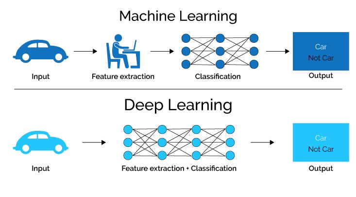
Figure 6.3: Comparison between Machine Learning & Deep Learning
There are three important types of neural networks that are also called pre-trained models in deep learning: Artificial Neural Networks (ANN), Convolution Neural Networks (CNN), and Recurrent Neural Networks (RNN). We will not use them but it is good to understand what are they.
In practice, predictive models used in a Data Science project are mostly mathematics formulated models. They are implemented in different computer programs with different languages. They are normally packed into integrated software packages. This software undertakes a mixture of training data and goes through number crunching, parameter adjustment, and error correction, which normally called trial or training, and finally produces a working prediction model. During the process of machine generating model, human involvement is much less but needed. It enables fine-tune the model and improving its performance. ### Model Validation {-}
A major problem in building models is that it is relatively easy to build a prediction model but it is not easy to prove the model is useful. That is to say, finding relationships that exist and are the result of random patterns in the training and testing datasets, but this relationship may not exist in the unseen datasets. Model validation is the task of confirming that the outputs of a model have enough fidelity to the outputs of the model building process that the objectives of the model can be achieved.
In practice, a model can be over-fitted or under-fitted. An over-fitted model can perform extremely well in the test with the test dataset but perform significantly worse with the new unseen dataset. In other words, the over-fitted model remembers a huge number of examples from the training dataset instead of learning to notice features of the training dataset. On other hand, an under-fitted model misses some features or patterns that exist in the training dataset. Under-fitting would occur, for example, when fitting a linear model to non-linear data. Both over-fitted and under-fitted models will tend to have poor predictive performance.
To determine if over-fitting has occurred, the model needs to be tested on “validation dataset”. Validation datasets are a subset from the given datasets that have targeted attributes values. This subset was not used to construct the model. The validation dataset is genially taken from the training datasets with a certain percentage.
Over-fitting is quite common and this is not necessarily a problem. However, if the degree of over-fitting is large, the model may need to be reconstructed using a different set of attributes.
Apart from checking the model’s over-fitting, Depends on the model being constructed, there a number of evaluation methods are available to perform the model validation such as Confusion Matrix for nominal output like class labels, AUC (Area Under Curve), Accuracy and other evaluation metrics are used for evaluating different models.
Correlation, in statistics, is a measurement of any statistical relationship between two attributes. It can be any association. It commonly refers to the degree to which a pair of attributes is linearly related.↩︎
The most commonly used measurement of the correlation between two attributes is the “Pearson’s correlation coefficient”, commonly called simply “the correlation coefficient”.↩︎
In statistics, step-wise linear regression is a method of fitting regression models in which the selection of predictors is carried out by a procedure that in each step, one attribute is considered for addition to or subtraction from the set of selected attributes based on some pre-specified criterion.↩︎
Principal component analysis (PCA) is the process of computing the principal components and using only the first few principal components and ignoring the rest in a prediction or data dimension reduction. The principal components are often computed by eigendecomposition of the data covariance matrix or singular value decomposition of the data matrix.↩︎