Chapter 8 Prediction with Decision Trees

Model building is the main task of any data science project after understood data, processed some attributes, and analysed the attributes’ correlations and the individual’s prediction power. As described in the previous chapters. There are many ways to build a prediction model. In this chapter, we will demonstrate to build a prediction model with the most simple algorithm - Decision tree.
A decision tree is a commonly used classification model, which is a flowchart-like tree structure. In a decision tree, each internal node (non-leaf node) denotes a test on an attribute, each branch represents an outcome of the test, and each leaf node (or terminal node) holds a class label. The topmost node in a tree is the root node. A typical decision tree is shown in Figure 8.1.
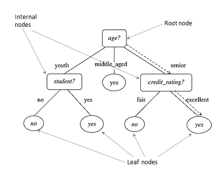
Figure 8.1: An example of decision tree
It represents the concept buys_computer, that is, it predicts whether a customer is likely to buy a computer or not. ‘yes’ is likely to buy, and ‘no’ is unlikely to buy. Internal nodes are denoted by rectangles, they are test conditions, and leaf nodes are denoted by ovals, which are the final predictions. Some decision trees produce binary trees where each internal node branches to exactly two other nodes. Others can produce non-binary trees, like age? in the above tree has three branches.
A decision tree is built by a process called tree induction, which is the learning or construction of decision trees from a class-labelled training dataset. Once a decision tree has been constructed, it can be used to classify a test dataset, which is also called deduction.
The deduction process is Starting from the root node of a decision tree, we apply the test condition to a record or data sample and follow the appropriate branch based on the outcome of the test. This will lead us either to another internal node, for which a new test condition is applied or to a leaf node. The class label associated with the leaf node is then assigned to the record or the data sample. For example, to predict a new data input with 'age=senior' and 'credit_rating=excellent', traverse starting from the root goes to the most right side along the decision tree and reaches a leaf yes, which is indicated by the dotted line in the figure 8.1.
Build a decision tree classifier needs to make two decisions:
- which attributes to use for test conditions?
- and in what order?
Answering these two questions differently forms different decision tree algorithms. Different decision trees can have different prediction accuracy on the test dataset. Some decision trees are more accurate and cheaper to run than others. Finding the optimal tree is computationally expensive and sometimes is impossible because of the exponential size of the search space. In real practice, it is often to seek efficient algorithms, that are reasonably accurate and only compute in a reasonable amount of time. Hunt’s, ID3, C4.5 and CART algorithms are all of this kind of algorithms for classification. The common feature of these algorithms is that they all employ a greedy strategy as demonstrated in the Hunt’s algorithm.