2.6 Prediction
The forecast of \(Y\) from \(X=x\) in the linear model is approached by two different ways:
- Inference on the conditional mean of \(Y\) given \(X=x\), \(\mathbb{E}[Y|X=x]\). This is a deterministic quantity, which equals \(\beta_0+\beta_1x\) in the linear model.
- Prediction of the conditional response \(Y|X=x\). This is a random variable, which in the linear model is distributed as \(\mathcal{N}(\beta_0+\beta_1x,\sigma^2)\).
Let’s study first the inference on the conditional mean. \(\beta_0+\beta_1x\) is estimated by \(\hat y=\hat\beta_0+\hat\beta_1x\). Then, is a deterministic quantity estimated by a random variable. Moreover, it can be shown that the \(100(1-\alpha)\%\) CI for \(\beta_0+\beta_1x\) is \[\begin{align} \left(\hat y \pm t_{n-2:\alpha/2}\sqrt{\frac{\hat\sigma^2}{n}\left(1+\frac{(x-\bar x)^2}{s_x^2}\right)}\right).\tag{2.9} \end{align}\] Some important remarks on (2.9) are:
Bias. The CI is centered around \(\hat y=\hat\beta_0+\hat\beta_1x\), which obviously depends on \(x\).
Variance. The variance that determines the length of the CI is \(\frac{\hat\sigma^2}{n}\left(1+\frac{(x-\bar x)^2}{s_x^2}\right)\). Its interpretation is very similar to the one given for \(\hat\beta_0\) and \(\hat\beta_1\) in Section 2.5:
- Sample size \(n\). As the sample size grows, the length of the CI decreases, since the estimates \(\hat\beta_0\) and \(\hat\beta_1\) become more precise.
- Error variance \(\sigma^2\). The more disperse \(Y\) is, the less precise \(\hat\beta_0\) and \(\hat\beta_1\) are, hence the more variance on estimating \(\beta_0+\beta_1x\).
- Predictor variance \(s_x^2\). If the predictor is spread out (large \(s_x^2\)), then it is easier to “anchor” the regression line. This helps on reducing the variance, but up to a certain limit: there is a variance component purely dependent on the error!
- Centrality \((x-\bar x)^2\). The more extreme \(x\) is, the wider the CI becomes. This is due to the “leverage” of the slope estimate \(\hat\beta_1\): a small deviation from the true \(\beta_1\) is magnified when \(x\) is far away from \(\bar x\), hence the more variability in these points. The minimum is achieved with \(x=\bar x\), but it does not correspond to zero variance.
Figure 2.23 helps visualizing these concepts interactively.
Figure 2.23: Illustration of the CIs for the conditional mean and response. Note how the length of the CIs is influenced by \(x\), specially for the conditional mean. Application also available here.
The prediction and computation of CIs can be done with the R function predict. The objects required for predict are: first, the output of lm; second, a data.frame containing the locations \(x\) where we want to predict \(\beta_0+\beta_1x\). To illustrate the use of predict, we are going to use the pisa dataset. In case you do not have it loaded, you can download it here as an .RData file.
# Plot the data and the regression line (alternatively, using R Commander)
scatterplot(MathMean ~ ReadingMean, data = pisa, smooth = FALSE)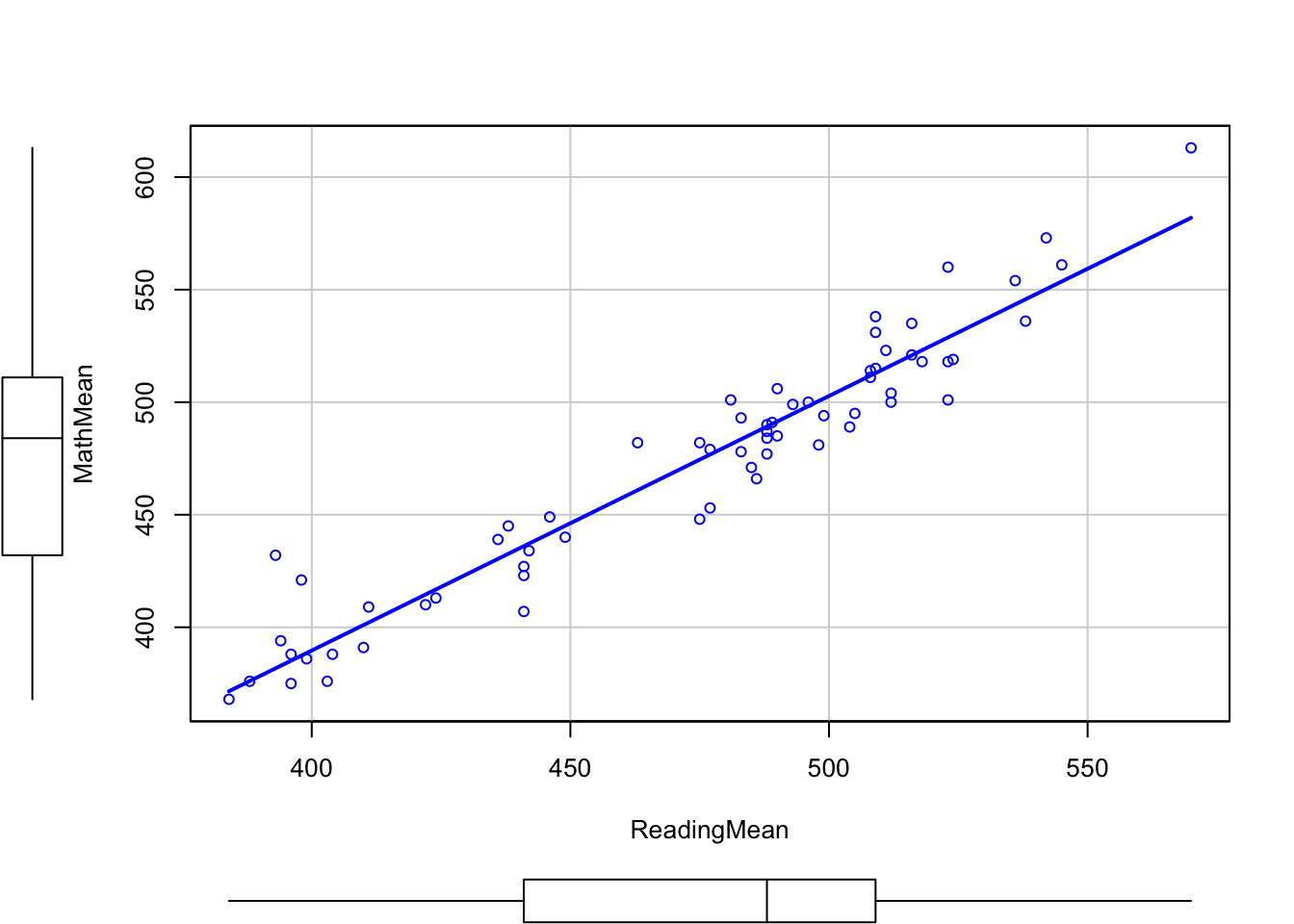
# Fit a linear model (alternatively, using R Commander)
model <- lm(MathMean ~ ReadingMean, data = pisa)
summary(model)
##
## Call:
## lm(formula = MathMean ~ ReadingMean, data = pisa)
##
## Residuals:
##     Min      1Q  Median      3Q     Max
## -29.039 -10.151  -2.187   7.804  50.241
##
## Coefficients:
##              Estimate Std. Error t value Pr(>|t|)
## (Intercept) -62.65638   19.87265  -3.153  0.00248 **
## ReadingMean   1.13083    0.04172  27.102  < 2e-16 ***
## ---
## Signif. codes:  0 '***' 0.001 '**' 0.01 '*' 0.05 '.' 0.1 ' ' 1
##
## Residual standard error: 15.72 on 63 degrees of freedom
## Multiple R-squared:  0.921,  Adjusted R-squared:  0.9198
## F-statistic: 734.5 on 1 and 63 DF,  p-value: < 2.2e-16

# Data for which we want a prediction for the mean
# Important! You have to name the column with the predictor name!
newData <- data.frame(ReadingMean = 400)

# Prediction
predict(model, newdata = newData)
##        1
## 389.6746

# Prediction with 95% confidence interval (the default)
# CI: (lwr, upr)
predict(model, newdata = newData, interval = "confidence")
##        fit      lwr     upr
## 1 389.6746 382.3782 396.971
predict(model, newdata = newData, interval = "confidence", level = 0.95)
##        fit      lwr     upr
## 1 389.6746 382.3782 396.971

# Other levels
predict(model, newdata = newData, interval = "confidence", level = 0.90)
##        fit      lwr    upr
## 1 389.6746 383.5793 395.77
predict(model, newdata = newData, interval = "confidence", level = 0.99)
##        fit      lwr      upr
## 1 389.6746 379.9765 399.3728

# Predictions for several values
summary(pisa$ReadingMean)
##    Min. 1st Qu.  Median    Mean 3rd Qu.    Max.
##     384     441     488     474     509     570
newData2 <- data.frame(ReadingMean = c(400, 450, 500, 550))
predict(model, newdata = newData2, interval = "confidence")
##        fit      lwr      upr
## 1 389.6746 382.3782 396.9710
## 2 446.2160 441.8363 450.5957
## 3 502.7574 498.2978 507.2170
## 4 559.2987 551.8587 566.7388
For the pisa dataset, do the following:
-
Regress
MathMeanonlogGDPpexcluding Shanghai-China, Vietnam and Qatar (usesubset = -c(1, 16, 62)). Name the fitted modelmodExercise. -
Show the scatterplot with regression line (use
subset = -c(1, 16, 62)). -
Compute the estimate for the conditional mean of
MathMeanfor alogGDPpof \(10.263\) (Spain’s). What is the CI at \(\alpha=0.05\)? -
Do the same with the
logGDPpof Sweden, Denmark, Italy and United States. -
Check that
modExercise$fitted.valuesis the same aspredict(modExercise, newdata = data.frame(logGDPp = pisa$logGDPp))(except for the three countries omitted). Why is so?
Let’s study now the prediction of the conditional response \(Y|X\). \(Y|X\) is predicted by \(\hat y=\hat\beta_0+\hat\beta_1x\) (the estimated conditional mean). So we estimate the unknown response \(Y|X\) simply by its conditional mean. This is clearly a different situation: now we estimate a random variable by another random variable. As a consequence, there is a price to pay in terms of extra variability and this is reflected in the \(100(1-\alpha)\%\) CI for \(Y|X\): \[\begin{align} \left(\hat y \pm t_{n-2:\alpha/2}\sqrt{\hat\sigma^2+\frac{\hat\sigma^2}{n}\left(1+\frac{(x-\bar x)^2}{s_x^2}\right)}\right)\tag{2.10} \end{align}\] The CI (2.10) is very similar to (2.9), but there is a key difference: it is always longer due to the extra term \(\hat\sigma^2\). In Figure 2.23 you can visualize the differences between both CIs.
Similarities and differences in the prediction of the conditional mean \(\mathbb{E}[Y|X=x]\) and conditional response \(Y|X=x\):
- Similarities. The estimate is the same, \(\hat y=\hat\beta_0+\hat\beta_1x\). Both CI are centered in \(\hat y\) and share the term \(\frac{\hat\sigma^2}{n}\left(1+\frac{(x-\bar x)^2}{s_x^2}\right)\) in the variance.
- Differences. \(\mathbb{E}[Y|X=x]\) is deterministic and \(Y|X=x\) is random. Therefore, the variance is larger for the prediction of \(Y|X=x\): there is an extra \(\hat\sigma^2\) term in the variance of its prediction.
The prediction and computation of CIs can be done with the R function predict. The objects required for predict are: first, the output of lm; second, a data.frame containing the locations \(x\) where we want to predict \(\beta_0+\beta_1 x\). To illustrate the use of predict, we are going to use the pisa dataset. In case you do not have it loaded, you can download it here as an .RData file.
The prediction of a new observation can be done via the function predict, which also provides confidence intervals.
# Prediction with 95% confidence interval (the default) CI: (lwr, upr)
predict(model, newdata = newData, interval = "prediction")
##        fit      lwr      upr
## 1 389.6746 357.4237 421.9255

# Other levels
predict(model, newdata = newData, interval = "prediction", level = 0.90)
##        fit      lwr      upr
## 1 389.6746 362.7324 416.6168
predict(model, newdata = newData, interval = "prediction", level = 0.99)
##        fit      lwr      upr
## 1 389.6746 346.8076 432.5417

# Predictions for several values
predict(model, newdata = newData2, interval = "prediction")
##        fit      lwr      upr
## 1 389.6746 357.4237 421.9255
## 2 446.2160 414.4975 477.9345
## 3 502.7574 471.0277 534.4870
## 4 559.2987 527.0151 591.5824

# Comparison with the mean CI
predict(model, newdata = newData2, interval = "confidence")
##        fit      lwr      upr
## 1 389.6746 382.3782 396.9710
## 2 446.2160 441.8363 450.5957
## 3 502.7574 498.2978 507.2170
## 4 559.2987 551.8587 566.7388
predict(model, newdata = newData2, interval = "prediction")
##        fit      lwr      upr
## 1 389.6746 357.4237 421.9255
## 2 446.2160 414.4975 477.9345
## 3 502.7574 471.0277 534.4870
## 4 559.2987 527.0151 591.5824
Redo the third and fourth points of the previous exercise with CIs for the conditional response. In addition, check if the MathMean scores of Sweden, Denmark, Vietnam and Qatar are inside or outside the prediction CIs.