4.1 More R basics

In order to implement some of the contents of this chapter we need to cover more R basics, mostly related with flexible plotting that is not implemented directly in R Commander. The R functions we will are also very useful for simplifying some R Commander approaches.

In the following sections, type – not copy and paste systematically – the code in the 'R Script' panel and send it to the output panel. Remember that you should get the same outputs (which are preceded by ## [1]).

4.1.1 Data frames revisited

# Let's begin importing the iris dataset
data(iris)

# names gives you the variables in the data frame
names(iris)
## [1] "Sepal.Length" "Sepal.Width"  "Petal.Length" "Petal.Width"  "Species"

# The beginning of the data
head(iris)
##   Sepal.Length Sepal.Width Petal.Length Petal.Width Species
## 1          5.1         3.5          1.4         0.2  setosa
## 2          4.9         3.0          1.4         0.2  setosa
## 3          4.7         3.2          1.3         0.2  setosa
## 4          4.6         3.1          1.5         0.2  setosa
## 5          5.0         3.6          1.4         0.2  setosa
## 6          5.4         3.9          1.7         0.4  setosa

# So we can access variables by $ or as in a matrix
iris$Sepal.Length[1:10]
##  [1] 5.1 4.9 4.7 4.6 5.0 5.4 4.6 5.0 4.4 4.9
iris[1:10, 1]
##  [1] 5.1 4.9 4.7 4.6 5.0 5.4 4.6 5.0 4.4 4.9
iris[3, 1]
## [1] 4.7

# Information on the dimension of the data frame
dim(iris)
## [1] 150   5

# str gives the structure of any object in R
str(iris)
## 'data.frame':    150 obs. of  5 variables:
##  $ Sepal.Length: num  5.1 4.9 4.7 4.6 5 5.4 4.6 5 4.4 4.9 ...
##  $ Sepal.Width : num  3.5 3 3.2 3.1 3.6 3.9 3.4 3.4 2.9 3.1 ...
##  $ Petal.Length: num  1.4 1.4 1.3 1.5 1.4 1.7 1.4 1.5 1.4 1.5 ...
##  $ Petal.Width : num  0.2 0.2 0.2 0.2 0.2 0.4 0.3 0.2 0.2 0.1 ...
##  $ Species     : Factor w/ 3 levels "setosa","versicolor",..: 1 1 1 1 1 1 1 1 1 1 ...

# Recall the species variable: it is a categorical variable (or factor),
# not a numeric variable
iris$Species[1:10]
##  [1] setosa setosa setosa setosa setosa setosa setosa setosa setosa setosa
## Levels: setosa versicolor virginica

# Factors can only take certain values
levels(iris$Species)
## [1] "setosa"     "versicolor" "virginica"

# If a file contains a variable with character strings as observations (either
# encapsulated by quotation marks or not), the variable will become a factor
# when imported into R

Do the following:

Import auto.txt into R as the data frame auto. Check how the character strings in the file give rise to factor variables.
Get the dimensions of auto and show beginning of the data.
Retrieve the fifth observation of horsepower in two different ways.
Compute the levels of name.

4.1.2 Vector-related functions

# The function seq creates sequences of numbers equally separated
seq(0, 1, by = 0.1)
##  [1] 0.0 0.1 0.2 0.3 0.4 0.5 0.6 0.7 0.8 0.9 1.0
seq(0, 1, length.out = 5)
## [1] 0.00 0.25 0.50 0.75 1.00

# You can short the latter argument
seq(0, 1, l = 5)
## [1] 0.00 0.25 0.50 0.75 1.00

# Repeat number
rep(0, 5)
## [1] 0 0 0 0 0

# Reverse a vector
myVec <- c(1:5, -1:3)
rev(myVec)
##  [1]  3  2  1  0 -1  5  4  3  2  1

# Another way
myVec[length(myVec):1]
##  [1]  3  2  1  0 -1  5  4  3  2  1

# Count repetitions in your data
table(iris$Sepal.Length)
## 
## 4.3 4.4 4.5 4.6 4.7 4.8 4.9   5 5.1 5.2 5.3 5.4 5.5 5.6 5.7 5.8 5.9   6 6.1 6.2 
##   1   3   1   4   2   5   6  10   9   4   1   6   7   6   8   7   3   6   6   4 
## 6.3 6.4 6.5 6.6 6.7 6.8 6.9   7 7.1 7.2 7.3 7.4 7.6 7.7 7.9 
##   9   7   5   2   8   3   4   1   1   3   1   1   1   4   1
table(iris$Species)
## 
##     setosa versicolor  virginica 
##         50         50         50

Do the following:

Create the vector \(x=(0.3, 0.6, 0.9, 1.2)\).
Create a vector of length 100 ranging from \(0\) to \(1\) with entries equally separated.
Compute the amount of zeros and ones in x <- c(0, 0, 1, 0, 1, 0, 0, 1, 0, 1, 0). Check that they are the same as in rev(x).
Compute the vector \((0.1, 1.1, 2.1, ..., 100.1)\) in four different ways using seq and rev. Do the same but using : instead of seq. (Hint: add 0.1)

4.1.3 Logical conditions and subsetting

# Relational operators: x < y, x > y, x <= y, x >= y, x == y, x!= y
# They return TRUE or FALSE

# Smaller than
0 < 1
## [1] TRUE

# Greater than
1 > 1
## [1] FALSE

# Greater or equal to
1 >= 1 # Remember: ">="" and not "=>"" !
## [1] TRUE

# Smaller or equal to
2 <= 1 # Remember: "<="" and not "=<"" !
## [1] FALSE

# Equal
1 == 1 # Tests equality. Remember: "=="" and not "="" !
## [1] TRUE

# Unequal
1 != 0 # Tests inequality
## [1] TRUE

# TRUE is encoded as 1 and FALSE as 0
TRUE + 1
## [1] 2
FALSE + 1
## [1] 1

# In a vector-like fashion
x <- 1:5
y <- c(0, 3, 1, 5, 2)
x < y
## [1] FALSE  TRUE FALSE  TRUE FALSE
x == y
## [1] FALSE FALSE FALSE FALSE FALSE
x != y
## [1] TRUE TRUE TRUE TRUE TRUE

# Subsetting of vectors
x
## [1] 1 2 3 4 5
x[x >= 2]
## [1] 2 3 4 5
x[x < 3]
## [1] 1 2

# Easy way of work with parts of the data
data <- data.frame(x = c(0, 1, 3, 3, 0), y = 1:5)
data
##   x y
## 1 0 1
## 2 1 2
## 3 3 3
## 4 3 4
## 5 0 5

# Data such that x is zero
data0 <- data[data$x == 0, ]
data0
##   x y
## 1 0 1
## 5 0 5

# Data such that x is larger than 2
data2 <- data[data$x > 2, ]
data2
##   x y
## 3 3 3
## 4 3 4

# In an example
iris$Sepal.Width[iris$Sepal.Width > 3]
##  [1] 3.5 3.2 3.1 3.6 3.9 3.4 3.4 3.1 3.7 3.4 4.0 4.4 3.9 3.5 3.8 3.8 3.4 3.7 3.6
## [20] 3.3 3.4 3.4 3.5 3.4 3.2 3.1 3.4 4.1 4.2 3.1 3.2 3.5 3.6 3.4 3.5 3.2 3.5 3.8
## [39] 3.8 3.2 3.7 3.3 3.2 3.2 3.1 3.3 3.1 3.2 3.4 3.1 3.3 3.6 3.2 3.2 3.8 3.2 3.3
## [58] 3.2 3.8 3.4 3.1 3.1 3.1 3.1 3.2 3.3 3.4

# Problem - what happened?
data[x > 2, ]
##   x y
## 3 3 3
## 4 3 4
## 5 0 5

# In an example
summary(iris)
##   Sepal.Length    Sepal.Width     Petal.Length    Petal.Width   
##  Min.   :4.300   Min.   :2.000   Min.   :1.000   Min.   :0.100  
##  1st Qu.:5.100   1st Qu.:2.800   1st Qu.:1.600   1st Qu.:0.300  
##  Median :5.800   Median :3.000   Median :4.350   Median :1.300  
##  Mean   :5.843   Mean   :3.057   Mean   :3.758   Mean   :1.199  
##  3rd Qu.:6.400   3rd Qu.:3.300   3rd Qu.:5.100   3rd Qu.:1.800  
##  Max.   :7.900   Max.   :4.400   Max.   :6.900   Max.   :2.500  
##        Species  
##  setosa    :50  
##  versicolor:50  
##  virginica :50  
##                 
##                 
## 
summary(iris[iris$Sepal.Width > 3, ])
##   Sepal.Length    Sepal.Width     Petal.Length    Petal.Width    
##  Min.   :4.400   Min.   :3.100   Min.   :1.000   Min.   :0.1000  
##  1st Qu.:5.000   1st Qu.:3.200   1st Qu.:1.450   1st Qu.:0.2000  
##  Median :5.400   Median :3.400   Median :1.600   Median :0.4000  
##  Mean   :5.684   Mean   :3.434   Mean   :2.934   Mean   :0.9075  
##  3rd Qu.:6.400   3rd Qu.:3.600   3rd Qu.:5.000   3rd Qu.:1.8000  
##  Max.   :7.900   Max.   :4.400   Max.   :6.700   Max.   :2.5000  
##        Species  
##  setosa    :42  
##  versicolor: 8  
##  virginica :17  
##                 
##                 
## 

# On the factor variable only makes sense == and !=
summary(iris[iris$Species == "setosa", ])
##   Sepal.Length    Sepal.Width     Petal.Length    Petal.Width   
##  Min.   :4.300   Min.   :2.300   Min.   :1.000   Min.   :0.100  
##  1st Qu.:4.800   1st Qu.:3.200   1st Qu.:1.400   1st Qu.:0.200  
##  Median :5.000   Median :3.400   Median :1.500   Median :0.200  
##  Mean   :5.006   Mean   :3.428   Mean   :1.462   Mean   :0.246  
##  3rd Qu.:5.200   3rd Qu.:3.675   3rd Qu.:1.575   3rd Qu.:0.300  
##  Max.   :5.800   Max.   :4.400   Max.   :1.900   Max.   :0.600  
##        Species  
##  setosa    :50  
##  versicolor: 0  
##  virginica : 0  
##                 
##                 
## 

# Subset argument in lm
lm(Sepal.Width ~ Petal.Length, data = iris, subset = Sepal.Width > 3)
## 
## Call:
## lm(formula = Sepal.Width ~ Petal.Length, data = iris, subset = Sepal.Width > 
##     3)
## 
## Coefficients:
##  (Intercept)  Petal.Length  
##      3.59439      -0.05455
lm(Sepal.Width ~ Petal.Length, data = iris, subset = iris$Sepal.Width > 3)
## 
## Call:
## lm(formula = Sepal.Width ~ Petal.Length, data = iris, subset = iris$Sepal.Width > 
##     3)
## 
## Coefficients:
##  (Intercept)  Petal.Length  
##      3.59439      -0.05455
# Both iris$Sepal.Width and Sepal.Width in subset are fine: data = iris
# tells R to look for Sepal.Width in the iris dataset

# Same thing for the subset field in R Commander's menus

# AND operator &
TRUE & TRUE
## [1] TRUE
TRUE & FALSE
## [1] FALSE
FALSE & FALSE
## [1] FALSE

# OR operator |
TRUE | TRUE
## [1] TRUE
TRUE | FALSE
## [1] TRUE
FALSE | FALSE
## [1] FALSE

# Both operators are useful for checking for ranges of data
y
## [1] 0 3 1 5 2
index1 <- (y <= 3) & (y > 0)
y[index1]
## [1] 3 1 2
index2 <- (y < 2) | (y > 4)
y[index2]
## [1] 0 1 5

# In an example
summary(iris[iris$Sepal.Width > 3 & iris$Sepal.Width < 3.5, ])
##   Sepal.Length    Sepal.Width     Petal.Length    Petal.Width   
##  Min.   :4.400   Min.   :3.100   Min.   :1.200   Min.   :0.100  
##  1st Qu.:4.925   1st Qu.:3.125   1st Qu.:1.500   1st Qu.:0.200  
##  Median :5.950   Median :3.200   Median :4.450   Median :1.400  
##  Mean   :5.781   Mean   :3.245   Mean   :3.460   Mean   :1.145  
##  3rd Qu.:6.700   3rd Qu.:3.400   3rd Qu.:5.375   3rd Qu.:2.075  
##  Max.   :7.200   Max.   :3.400   Max.   :6.000   Max.   :2.500  
##        Species  
##  setosa    :20  
##  versicolor: 8  
##  virginica :14  
##                 
##                 
##

Do the following for the iris dataset:

Compute the subset corresponding to Petal.Length either smaller than 1.5 or larger than 2. Save this dataset as irisPetal.
Compute and summarize a linear regression of Sepal.Width into Petal.Width + Petal.Length for the dataset irisPetal. What is the \(R^2\)? (Solution: 0.101)
Check that the previous model is the same as regressing Sepal.Width into Petal.Width + Petal.Length for the dataset iris with the appropriate subset expression.
Compute the variance for Petal.Width when Petal.Width is smaller or equal that 1.5 and larger than 0.3. (Solution: 0.1266541)

4.1.4 Plotting functions

# plot is the main function for plotting in R
# It has a different behavior depending on the kind of object that it receives

# For example, for a regression model, it produces diagnostic plots
mod <- lm(Sepal.Width ~ Sepal.Length, data = iris)
plot(mod, 1)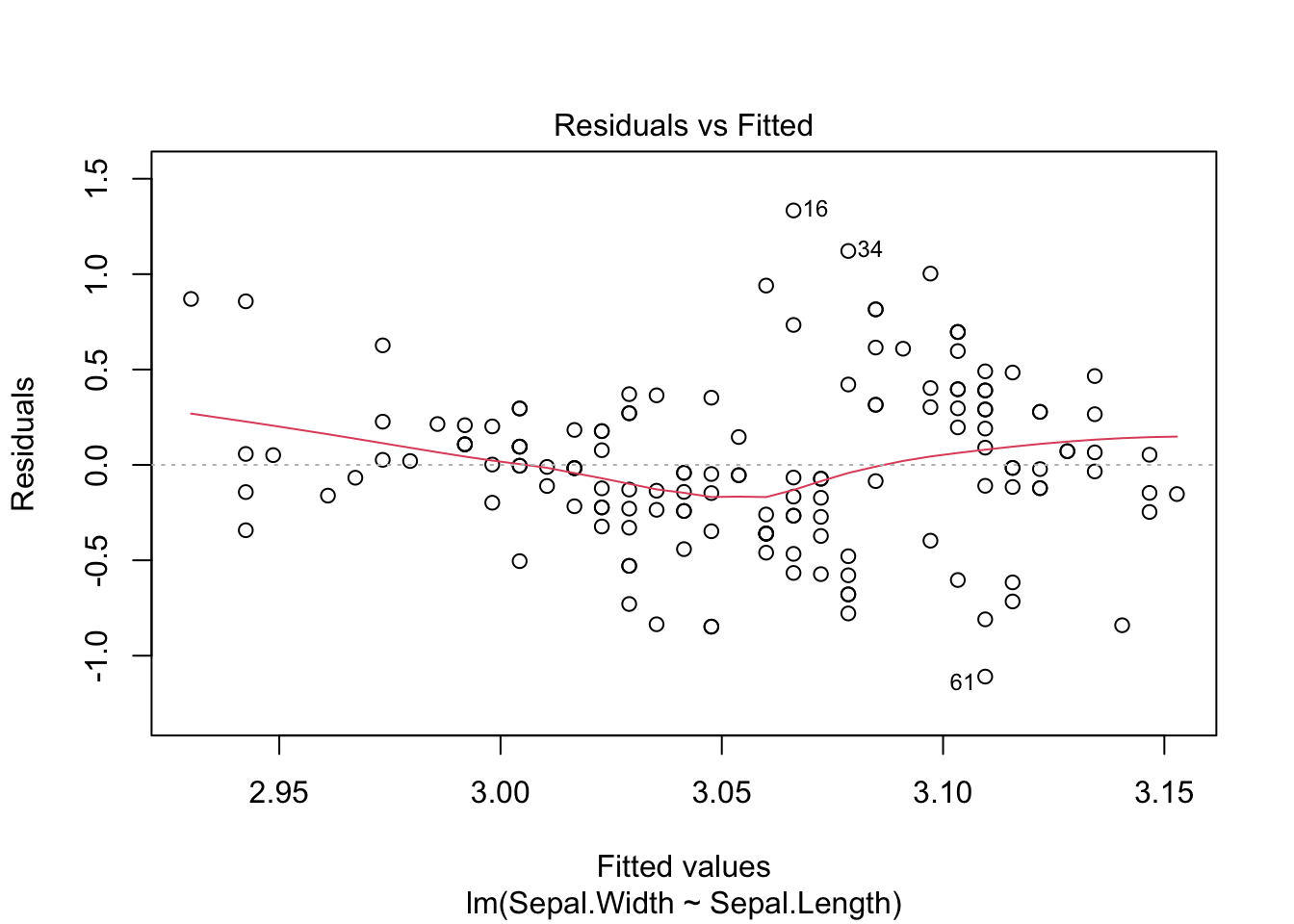


# How to plot some data
plot(iris$Sepal.Length, iris$Sepal.Width, main = "Sepal.Length vs Sepal.Width")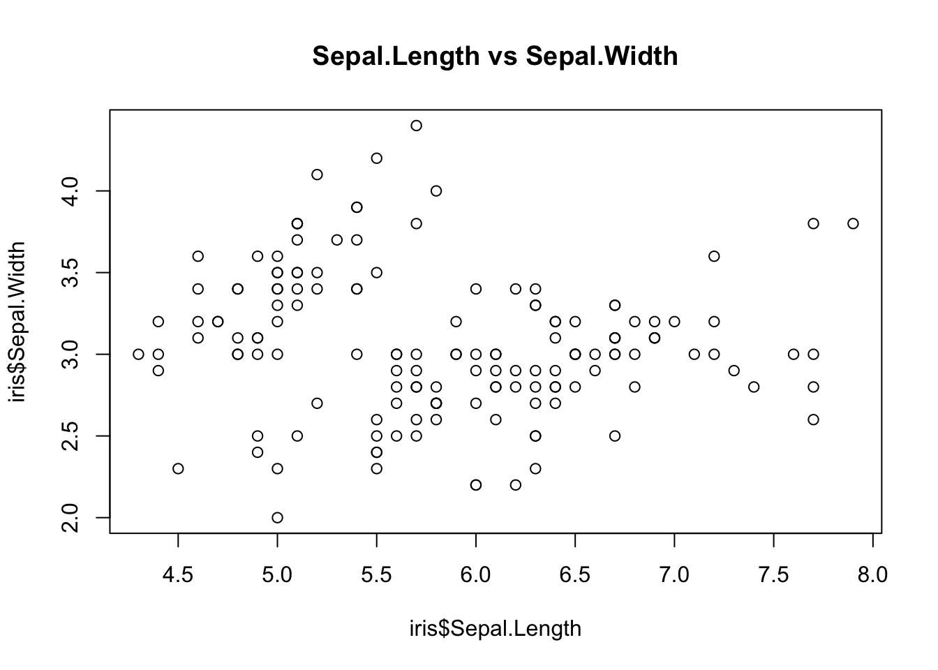


# Change the axis limits
plot(iris$Sepal.Length, iris$Sepal.Width, xlim = c(0, 10), ylim = c(0, 10))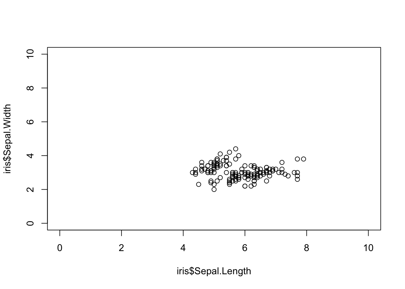


# How to plot a curve (a parabola)
x <- seq(-1, 1, l = 50)
y <- x^2
plot(x, y)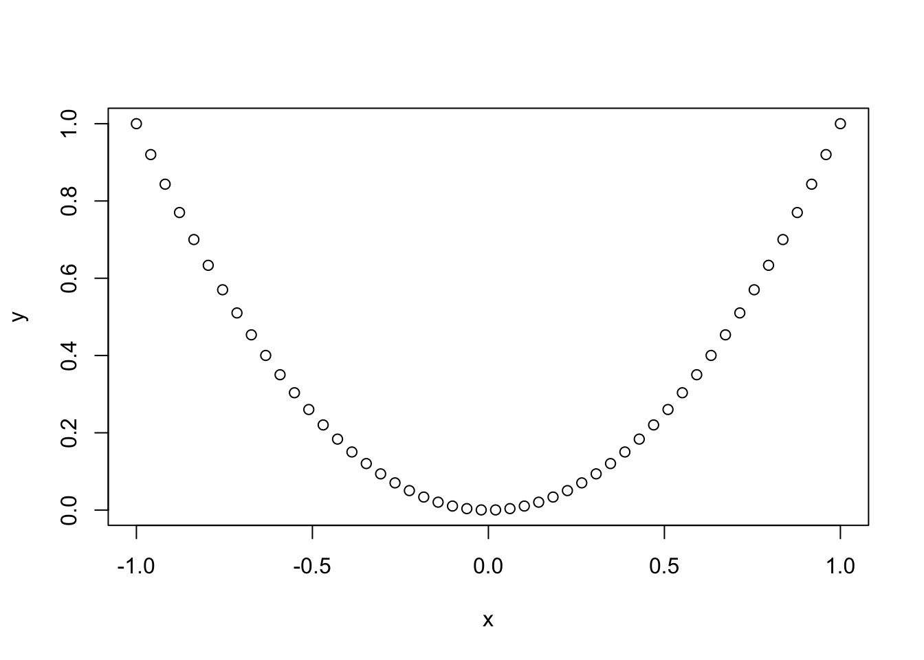

plot(x, y, main = "A dotted parabola")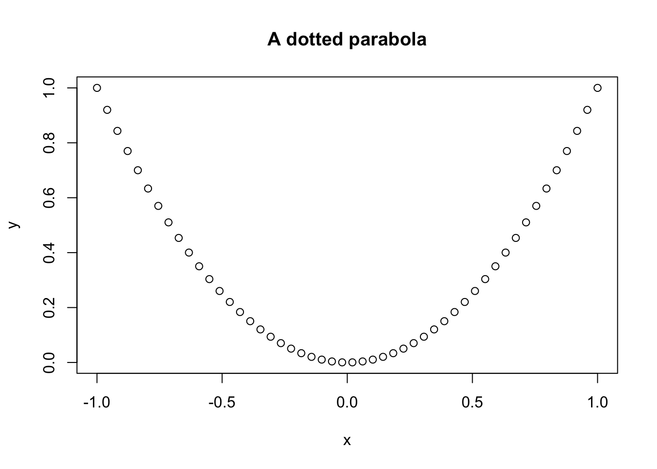

plot(x, y, main = "A parabola", type = "l")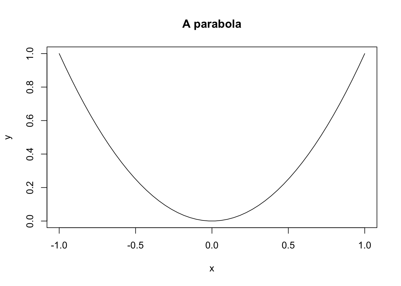

plot(x, y, main = "A red and thick parabola", type = "l", col = "red", lwd = 3)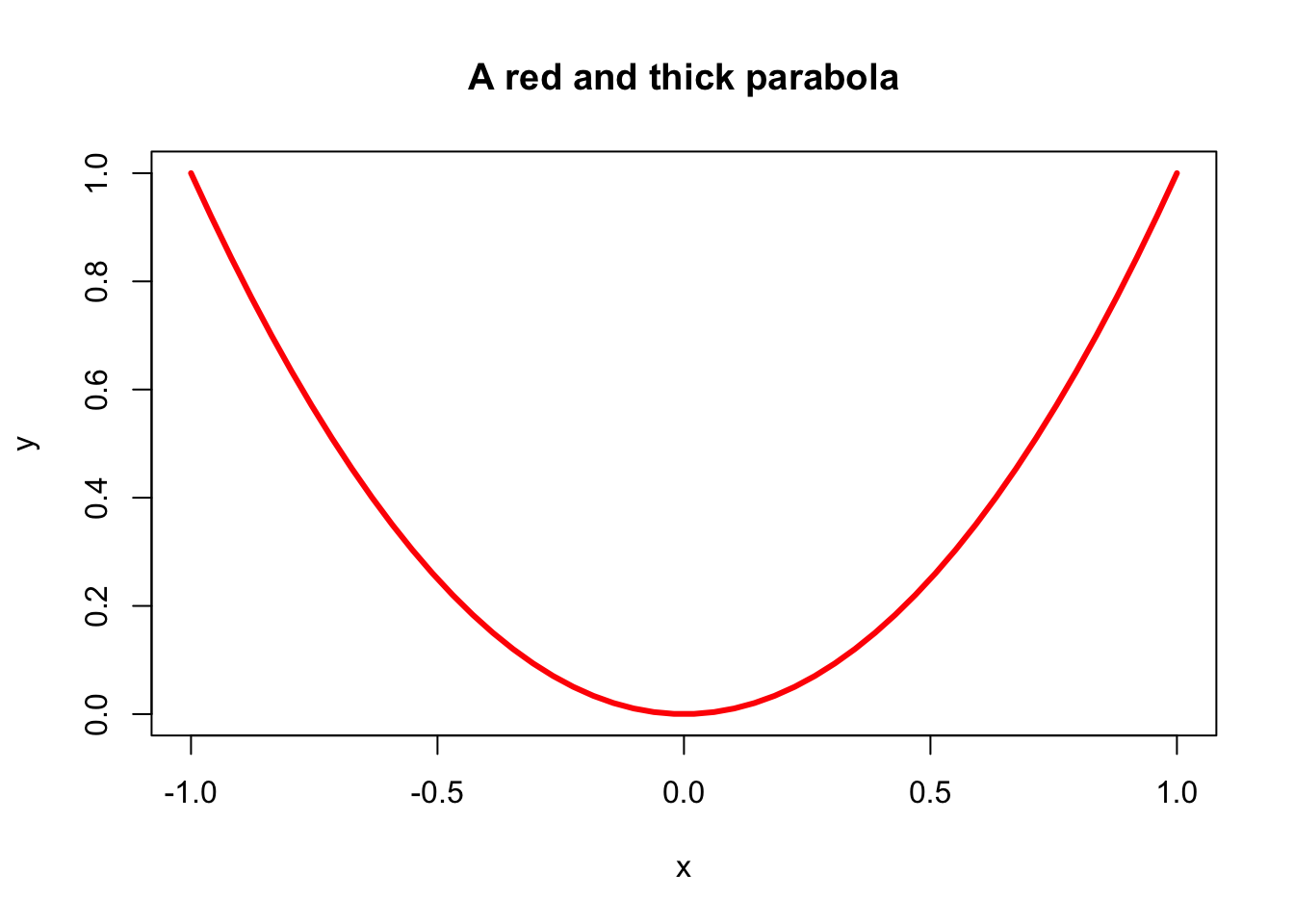


# Plotting a more complicated curve between -pi and pi
x <- seq(-pi, pi, l = 50)
y <- (2 + sin(10 * x)) * x^2
plot(x, y, type = "l") # Kind of rough...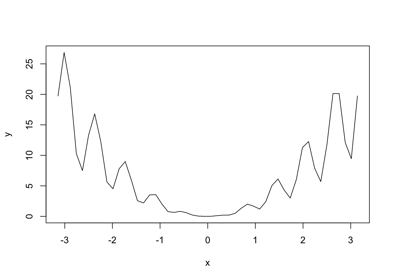


# More detailed plot
x <- seq(-pi, pi, l = 500)
y <- (2 + sin(10 * x)) * x^2
plot(x, y, type = "l")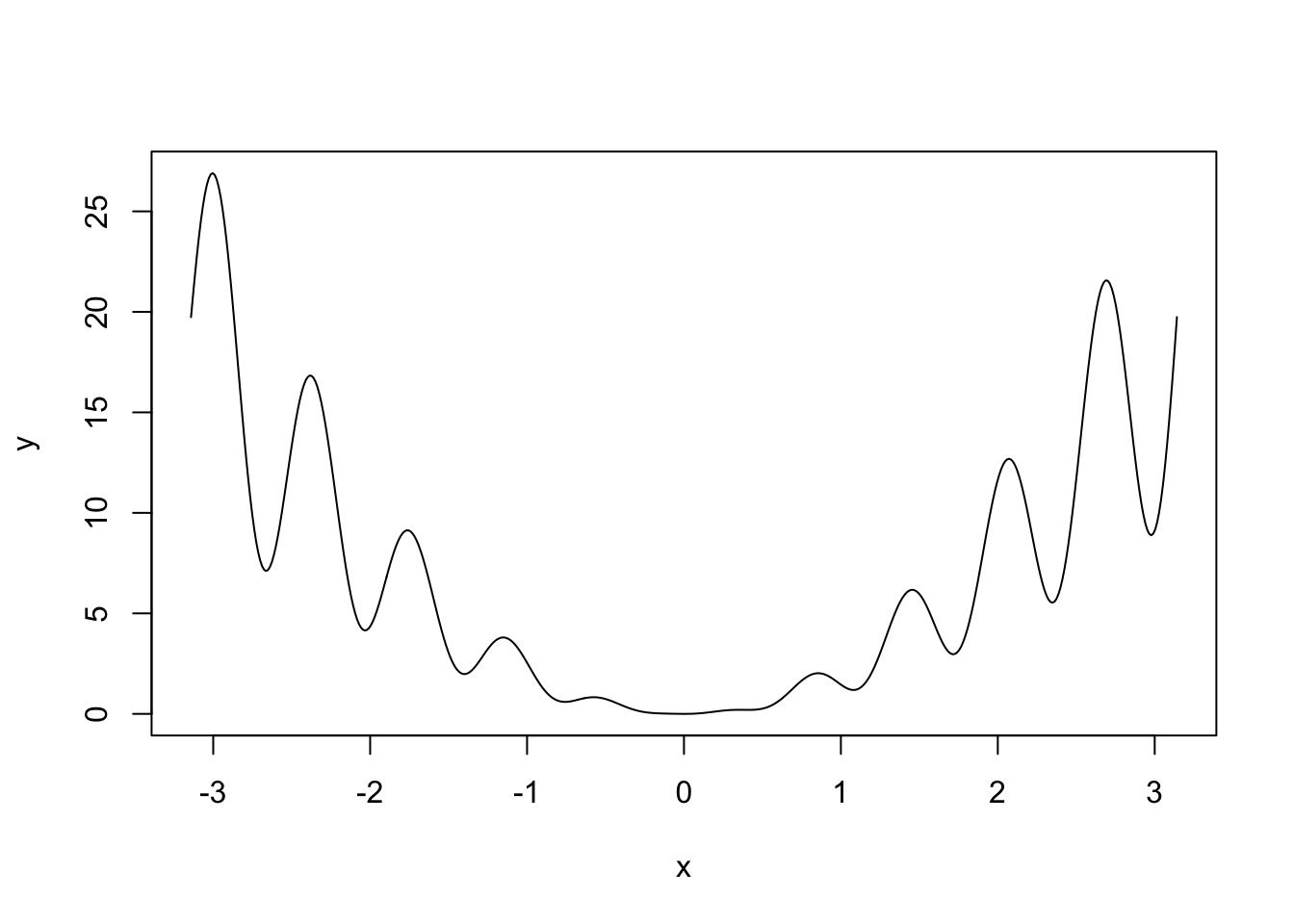


# Remember that we are joining points for creating a curve!

# For more options in the plot customization see
?plot
## Help on topic 'plot' was found in the following packages:
## 
##   Package               Library
##   base                  /Library/Frameworks/R.framework/Resources/library
##   graphics              /Library/Frameworks/R.framework/Versions/4.1-arm64/Resources/library
## 
## 
## Using the first match ...
?par

# plot is a first level plotting function. That means that whenever is called,
# it creates a new plot. If we want to add information to an existing plot, we
# have to use a second level plotting function such as points, lines or abline

plot(x, y) # Create a plot
lines(x, x^2, col = "red") # Add lines
points(x, y + 10, col = "blue") # Add points
abline(a = 5, b = 1, col = "orange", lwd = 2) # Add a straight line y = a + b * x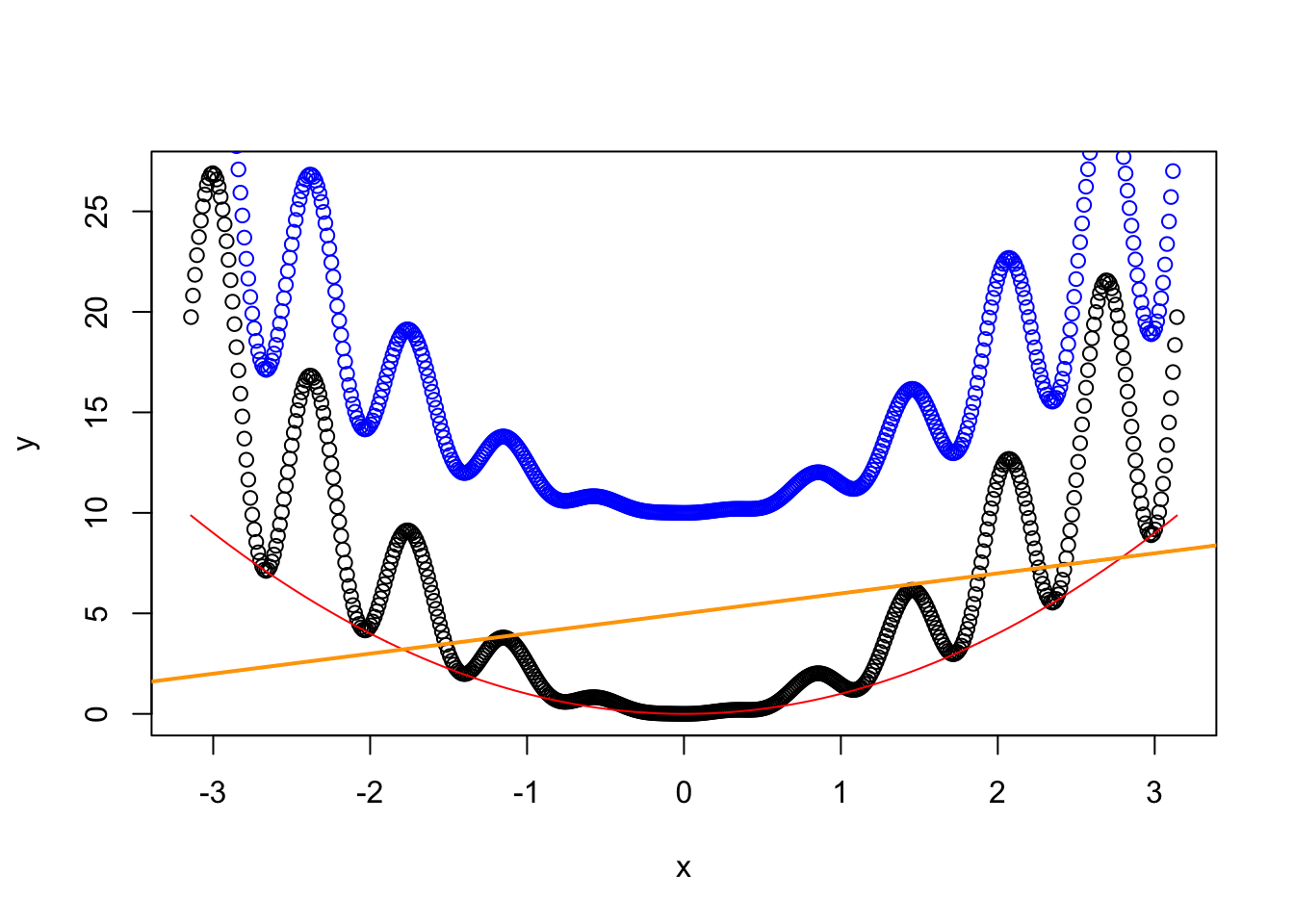

4.1.5 Distributions

The operations on distributions described here are implemented in R Commander through the menu 'Distributions', but is convenient for you to grasp how are they working.

# R allows to sample [r], compute density/probability mass [d],
# compute distribution function [p] and compute quantiles [q] for several
# continuous and discrete distributions. The format employed is [rdpq]name,
# where name stands for:
# - norm -> Normal
# - unif -> Uniform
# - exp -> Exponential
# - t -> Student's t
# - f -> Snedecor's F
# - chisq -> Chi squared
# - pois -> Poisson
# - binom -> Binomial
# More distributions:
?Distributions

# Sampling from a Normal - 100 random points from a N(0, 1)
rnorm(n = 10, mean = 0, sd = 1)
##  [1] -1.8367426 -1.3366952 -0.4906582  1.0215158  0.1637865  2.5039127
##  [7]  1.3113124 -0.1352548  0.1846896 -0.6373963

# If you want to have always the same result, set the seed of the random number
# generator
set.seed(45678)
rnorm(n = 10, mean = 0, sd = 1)
##  [1]  1.4404800 -0.7195761  0.6709784 -0.4219485  0.3782196 -1.6665864
##  [7] -0.5082030  0.4433822 -1.7993868 -0.6179521

# Plotting the density of a N(0, 1) - the Gauss bell
x <- seq(-4, 4, l = 100)
y <- dnorm(x = x, mean = 0, sd = 1)
plot(x, y, type = "l")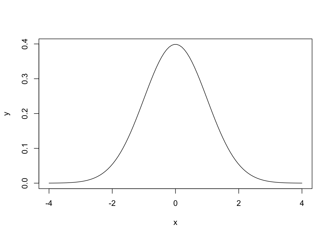


# Plotting the distribution function of a N(0, 1)
x <- seq(-4, 4, l = 100)
y <- pnorm(q = x, mean = 0, sd = 1)
plot(x, y, type = "l")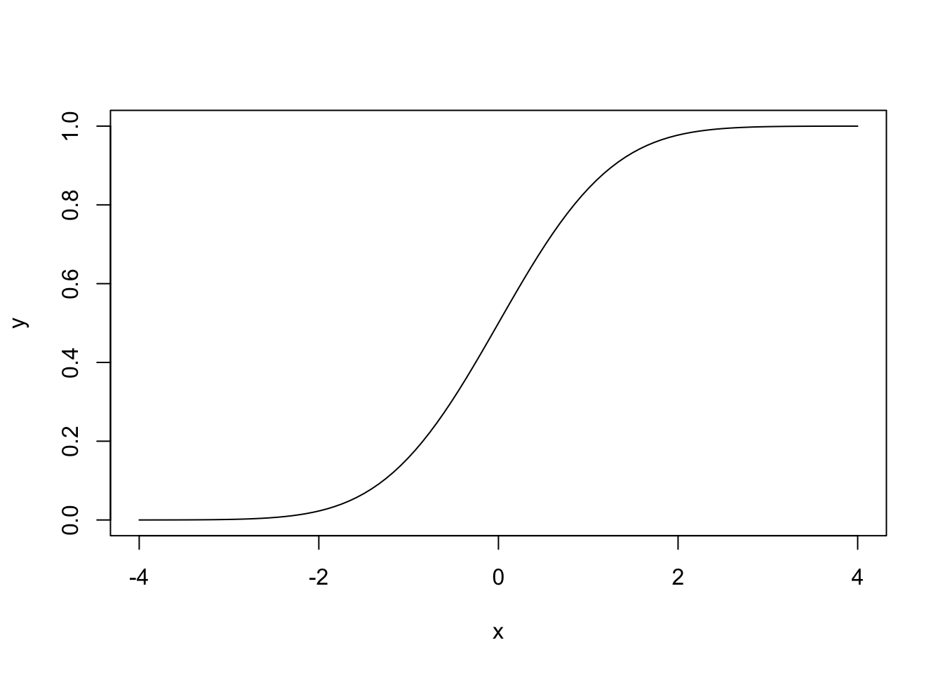


# Computing the 95% quantile for a N(0, 1)
qnorm(p = 0.95, mean = 0, sd = 1)
## [1] 1.644854

# All distributions have the same syntax: rname(n,...), dname(x,...), dname(p,...)  
# and qname(p,...), but the parameters in ... change. Look them in ?Distributions
# For example, here is the same for the uniform distribution

# Sampling from a U(0, 1)
set.seed(45678)
runif(n = 10, min = 0, max = 1)
##  [1] 0.9251342 0.3339988 0.2358930 0.3366312 0.7488829 0.9327177 0.3365313
##  [8] 0.2245505 0.6473663 0.0807549

# Plotting the density of a U(0, 1)
x <- seq(-2, 2, l = 100)
y <- dunif(x = x, min = 0, max = 1)
plot(x, y, type = "l")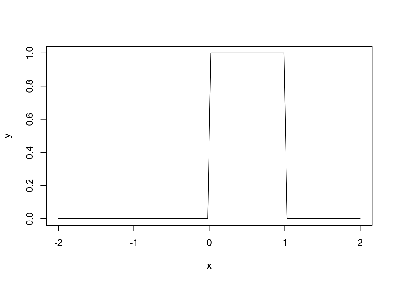


# Computing the 95% quantile for a U(0, 1)
qunif(p = 0.95, min = 0, max = 1)
## [1] 0.95

# Sampling from a Bi(10, 0.5)
set.seed(45678)
samp <- rbinom(n = 200, size = 10, prob = 0.5)
table(samp) / 200
## samp
##     1     2     3     4     5     6     7     8     9 
## 0.010 0.060 0.115 0.220 0.210 0.215 0.115 0.045 0.010

# Plotting the probability mass of a Bi(10, 0.5)
x <- 0:10
y <- dbinom(x = x, size = 10, prob = 0.5)
plot(x, y, type = "h") # Vertical bars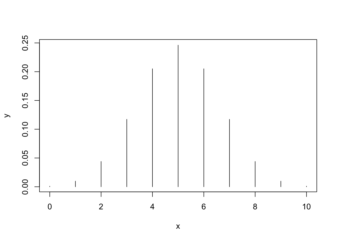


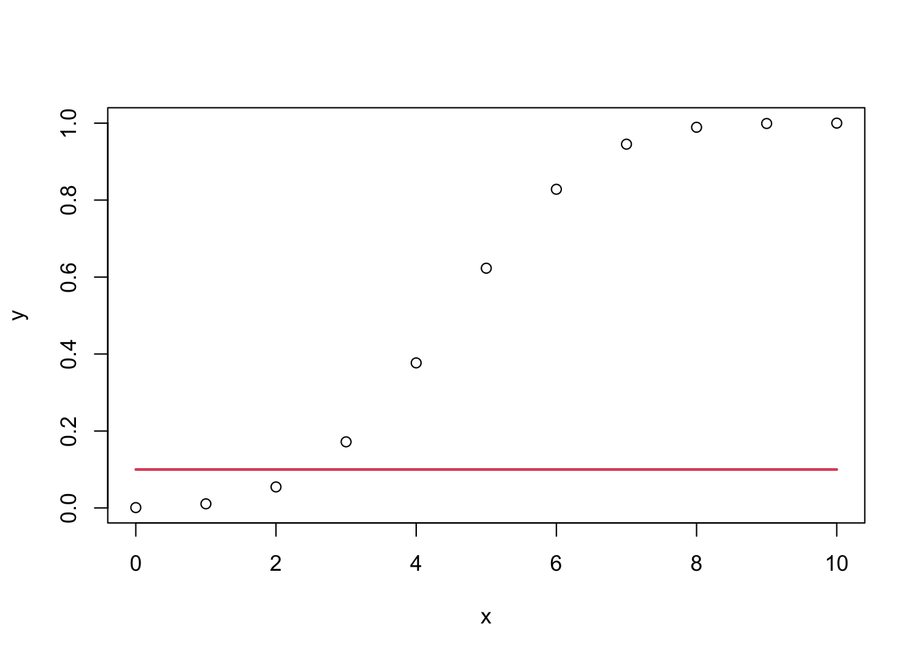
# Plotting the distribution function of a Bi(10, 0.5)
x <- 0:10
y <- pbinom(q = x, size = 10, prob = 0.5)
plot(x, y, type = "h")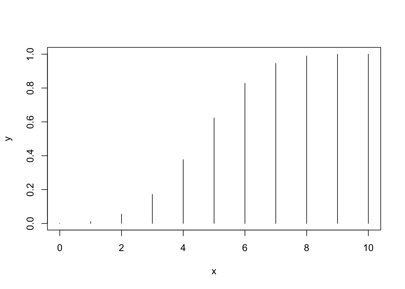

Do the following:

Compute the 90%, 95% and 99% quantiles of a \(F\) distribution with df1 = 1 and df2 = 5. (Answer: c(4.060420, 6.607891, 16.258177))
Plot the distribution function of a \(U(0,1)\). Does it make sense with its density function?
Sample 100 points from a Poisson with lambda = 5.
Sample 100 points from a \(U(-1,1)\) and compute its mean.
Plot the density of a \(t\) distribution with df = 1 (use a sequence spanning from -4 to 4). Add lines of different colors with the densities for df = 5, df = 10, df = 50 and df = 100. Do you see any pattern?

4.1.6 Defining functions

# A function is a way of encapsulating a block of code so it can be reused easily
# They are useful for simplifying repetitive tasks and organize the analysis
# For example, in Section 3.7 we had to make use of simpleAnova for computing
# the simple ANOVA table in multiple regression.

# This is a silly function that takes x and y and returns its sum
add <- function(x, y) {
  x + y
}

# Calling add - you need to run the definition of the function first!
add(1, 1)
## [1] 2
add(x = 1, y = 2)
## [1] 3

# A more complex function: computes a linear model and its posterior summary.
# Saves us a few keystrokes when computing a lm and a summary
lmSummary <- function(formula, data) {
  model <- lm(formula = formula, data = data)
  summary(model)
}

# Usage
lmSummary(Sepal.Length ~ Petal.Width, iris)
## 
## Call:
## lm(formula = formula, data = data)
## 
## Residuals:
##      Min       1Q   Median       3Q      Max 
## -1.38822 -0.29358 -0.04393  0.26429  1.34521 
## 
## Coefficients:
##             Estimate Std. Error t value Pr(>|t|)    
## (Intercept)  4.77763    0.07293   65.51   <2e-16 ***
## Petal.Width  0.88858    0.05137   17.30   <2e-16 ***
## ---
## Signif. codes:  0 '***' 0.001 '**' 0.01 '*' 0.05 '.' 0.1 ' ' 1
## 
## Residual standard error: 0.478 on 148 degrees of freedom
## Multiple R-squared:  0.669,  Adjusted R-squared:  0.6668 
## F-statistic: 299.2 on 1 and 148 DF,  p-value: < 2.2e-16

# Recall: there is no variable called model in the workspace.
# The function works on its own workspace!
model
## 
## Call:
## lm(formula = medv ~ crim + lstat + zn + nox, data = Boston)
## 
## Coefficients:
## (Intercept)         crim        lstat           zn          nox  
##    30.93462     -0.08297     -0.90940      0.03493      5.42234

# Add a line to a plot
addLine <- function(x, beta0, beta1) {
  lines(x, beta0 + beta1 * x, lwd = 2, col = 2)
}

# Usage
plot(x, y)
addLine(x, beta0 = 0.1, beta1 = 0)