2.9 Exercises and case studies

2.9.1 Data importation

Import the following datasets into R Commander indicating the right formatting options:

Create the file datasets.RData for saving all the datasets together.

There are a good number of datasets directly available in R:

To inspect them, go to ‘Data’ -> ‘Data in packages’ -> ‘List datasets in packages’ and you will get a long list of the available datasets, the package where they are stored and a small description about them. Or, in R, simply type data().
To load a dataset, go to ‘Data’ -> ‘Data in packages’ -> ‘Read dataset from an attached package…’ and select the package and dataset. Or, in R, simply type data(nameDataset, package = “namePackage”).
To get help on the dataset, go to ‘Help’ -> ‘Help on active dataset (if available)’ or simply type help(nameDataset).

As you can see, this is a handy way of accessing a good number of datasets directly from R.

Import the datasets Titanic (datasets package), PublicSchools (sandwich package) and USArrests (datasets package). Describe briefly the characteristics of each dataset (dimensions, variables, context).

2.9.2 Simple data management

Perform the following data management operations. Remember to select the adequate dataset as the active one:

Load datasets.RData.
Establish the case names in la-liga-2015-2016 as the variable Team (if they were not set).
Establish the case names in wdi-countries as the variable Country.
In la-liga-2015-2016, create a new variable named Goals.wrt.mean, defined as Goals - mean(Goals).
In wdi-countries, create a new variable that standardizes¹⁶ the GDP.growth. Call it GDP.growth.
Delete the variable Species from iris.
For la-liga-2015-2016, go to 'Edit dataset' and change the Points of Getafe to 40. To do so, click on the cell, change the content and click OK or select a new cell to save changes. Do not hit 'Enter’ or you will add a new column!.
Explore the menu options of 'Edit dataset'for adding and removing rows/columns. Is a useful feature for simple edits.
Create a newDatasets.RData file saving all the modified datasets.
Restart R Commander and then load newDatasets.RData (ignore the error 'ERROR: There is more than one object in the file...' and check that all the datasets are indeed available).

2.9.3 Computing simple linear regressions

Import the iris dataset, either from iris.txt or datasets.RData. This dataset contains measurements for 150 iris flowers. The purpose of this exercise is to do the following analyses through R Commander while inspecting and understanding the outputted code to identify what parts are changing, how and why.

Fit the regression line for Petal.Width (response) on Petal.Length (predictor) and summarize it.
Make the scatterplot of Petal.Width (y) vs. Petal.Length (x) with a regression line.
Set the ‘Graph title’ to “iris dataset: petal width vs. petal length,” the ‘x-axis label’ to “petal length” and ‘y-axis label’ to “sepal length.”
Identify the 5 most outlier points ‘Automatically’.
Redo the linear regression and scatterplot excluding the points labeled as outliers (exclude them in ‘Subset expression’ with a -c(…)).
Check that the summary for the fitted line and the scatterplot displayed are coherent.
Make the matrix scatterplot for the four variables and including ‘Least-squares lines’.
Set the ‘On Diagonal’ plots to ‘Histograms’ and ‘Boxplots’.
Set the ‘Graph title’ to “iris matrix scatterplot.”
Identify the 5 most outlier points ‘Automatically’.
Modify the code to identify 15 points.
Compute the regression line for the plot in the fourth row and the second column and create the scatterplot for it.
Redo the scatterplot by selecting the option ‘Plot by groups…’ and then selecting ‘Species’.

The last scatterplots are an illustration of the Simpson’s paradox. The paradox surges when there are two or more well-defined groups in the data, they all have positive (negative) correlation, but taken as a whole dataset, the correlation is the opposite.

2.9.4 R basics

Answer briefly in your own words:

What is the operator <- doing? What does it mean, for example, that a <- 1:5?
What is the difference between a matrix and a data frame? Why is the latter useful?
What are the differences between a vector and a matrix?
What is c employed for?
Consider the expression lm(a ~ b, data = myData).
- What is lm standing for?
- What does it mean a ~ b? What are the roles of a and b?
- Is myData a matrix or a data frame?
- What must be the relation between myData and a and b?
- Explain the differences with lm(b ~ a, data = myData).
What are the differences between running a <- 1; a, a <- 1 and 1.
What are the differences between a list and a data frame? What are their common parts?
Why is $ employed? How can you know in which variables you can use $?
If you have a vector x, what are x^2 and x + 1 doing to its elements?

Do the following:

Create the vectors $x = (1.17, 0.41, 0.34, 1.11, 1.02, 0.22, -0.24, -0.27, -0.40, -1.38)$ and $y = (3.63, 1.69, 0.27, 5.83, 2.64, 1.33, 1.22 -0.62, 1.29, -0.43)$.
Set the positions 3, 4 and 8 of $x$ to 0. Set the positions 1, 4, 9 of $y$ to 0.5, -0.75 and 0.3, respectively.
Create a new vector $z$ containing $\log(x^2) - y^3\sqrt{\exp(x)}$.
Create the vector $t=(1, 4, 9, 16, 25, \ldots, 100)$.
Access all the elements of $t$ except the third and fifth.
Create the matrix $A=\begin{pmatrix}1 & -3\\0 & 2\end{pmatrix}$. Hint: use rbind or cbind.
Using $A$, what is a short way (less amount of code) of computing $B=\begin{pmatrix}1+\sqrt{2}\sin(3) & -3+\sqrt{2}\sin(3)\\0+\sqrt{2}\sin(3) & 2+\sqrt{2}\sin(3)\end{pmatrix}$?
Compute A*B. Check that it makes sense with the results of A[1, 1] * B[1, 1], A[1, 2] * B[1, 2], A[2, 1] * B[2, 1] and A[2, 2] * B[2, 2]. Why?
Create a data frame named worldPopulation such that:
- the first variable is called Year and contains the values c(1915, 1925, 1935, 1945, 1955, 1965, 1975, 1985, 1995, 2005, 2015).
- the second variable is called Population and contains the values c(1798.0, 1952.3, 2197.3, 2366.6, 2758.3, 3322.5, 4061.4, 4852.5, 5735.1, 6519.6, 7349.5).
Write names(worldPopulation). Access to the two variables.
Create a new variable in worldPopulation called logPopulation that contains log(Population).
Compute the standard deviation, mean and median of the variables in worldPopulation.
Regress logPopulation into Year. Save the result as mod.
Compute the summary of the model and save it as sumMod.
Do a str on A, worldPopulation, mod and sumMod.
Access the $R^2$ and $\hat\sigma$ in sumMod.
Check that $R^2$ is the same as the squared correlation between predictor and response, and also the squared correlation between response and mod$fitted.values.

2.9.5 Model formulation and estimation

Answer the following conceptual questions in your own words:

What is the difference between $(\beta_0,\beta_1)$ and $(\hat\beta_0,\hat\beta_1)$.
Is $\hat\beta_0$ a random variable? What about $\hat\beta_1$? Justify your answer.
What function are the least squares estimates minimizing? Is important the choice of the kind distances (horizontal, vertical, perpendicular)?
What is the justification for the use of a vertical distance in the RSS?
Is $\sigma^2$ affecting the $R^2$ (indirectly or directly)? Why?
What are the residuals? What is their interpretation?
What are the fitted values? What is their interpretation?
What is the relation of $\hat \beta_1$ with $r_{xy}$?

Finally, check that the regression line goes through $(\bar X, \bar Y)$, in other words, that $\bar Y=\hat\beta_0+\hat\beta_1\bar X$.

2.9.6 Assumptions of the linear model

The dataset moreAssumptions.RData (download) contains the variables x1, …, x9 and y1, …, y9. For each regression y1 ~ x1, …, y9 ~ x9 describe whether the assumptions of the linear model are being satisfied or not. Justify your answer and state which assumption(s) you think are violated.

2.9.7 Nonlinear relations

Load moreAssumptions. For the regressions y1 ~ x1, y2 ~ x2, y6 ~ x6 and y9 ~ x9, identify which nonlinear transformation yields the largest $R^2$. For that transformation, check wether the assumptions are verified.

Hints: use the transformations in Figure 2.26 for the three first regressions. For y9 ~ x9, try with (5 - x9)^2, abs(x9 - 5) and abs(x9 - 5)^3.

2.9.8 Case study: Moore’s law

Moore’s law (Moore 1965) is an empirical law that states that the power of a computer doubles approximately every two years. More precisely:

Moore’s law is the observation that the number of transistors in a dense integrated circuit [e.g. a CPU] doubles approximately every two years.

— Wikipedia article on Moore’s law

Translated into a mathematical formula, Moore’s law is \[\begin{align*} \text{transistors}\approx 2^{\text{years}/2}. \end{align*}\] Applying logarithms to both sides gives (why?) \[\begin{align*} \log(\text{transistors})\approx \frac{\log(2)}{2}\text{years}. \end{align*}\] We can write the above formula more generally \[\begin{align*} \log(\text{transistors})=\beta_0+\beta_1 \text{years}+\varepsilon, \end{align*}\] where $\varepsilon$ is a random error. This is a linear model!

The dataset cpus.txt (download) contains the transistor counts for the CPUs appeared in the time range 1971–2015. For this data, do the following:

Import conveniently the data and name it as cpus.
Show a scatterplot of Transistor.count vs. Date.of.introduction with a linear regression.
Are the assumptions verified in Transistor.count ~ Date.of.introduction? Which ones are which are more “problematic?”
Create a new variable, named Log.Transistor.count, containing the logarithm of Transistor.count.
Show a scatterplot of Log.Transistor.count vs. Date.of.introduction with a linear regression.
Are the assumptions verified in Log.Transistor.count ~ Date.of.introduction? Which ones are which are more “problematic?”
Regress Log.Transistor.count ~ Date.of.introduction.
Summarize the fit. What are the estimates $\hat\beta_0$ and $\hat\beta_1$? Is $\hat\beta_1$ close to $\frac{\log(2)}{2}$?
Compute the CI for $\beta_1$ at $\alpha=0.05$. Is $\frac{\log(2)}{2}$ inside it? What happens at levels $\alpha=0.10,0.01$?
We want to forecast the average log-number of transistors for the CPUs to be released in 2017. Compute the adequate prediction and CI.
A new CPU design is expected for 2017. What is the range of log-number of transistors expected for it, at a 95% level of confidence?
Compute the ANOVA table for Log.Transistor.count ~ Date.of.introduction. Is $\beta_1$ significative?

The dataset gpus.txt (download) contains the transistor counts for the GPUs appeared in the period 1997–2016. Repeat the previous analysis for this dataset.

2.9.9 Case study: Growth in a time of debt

In the aftermath of the 2007–2008 financial crisis, the paper Growth in a time of debt (Reinhart and Rogoff 2010), from Carmen M. Reinhart and Kenneth Rogoff (both at Harvard), provided an important economical support for pro-austerity policies. The paper claimed that for levels of external debt in excess of 90% of the GDP, the GDP growth of a country was dramatically different than for lower levels of external debt. Therefore, it concludes the existence of a magical threshold – 90% – for which the level of external debt must be kept below in order to have a growing economy. Figure 2.29, extracted from Reinhart and Rogoff (2010), illustrates the main finding.

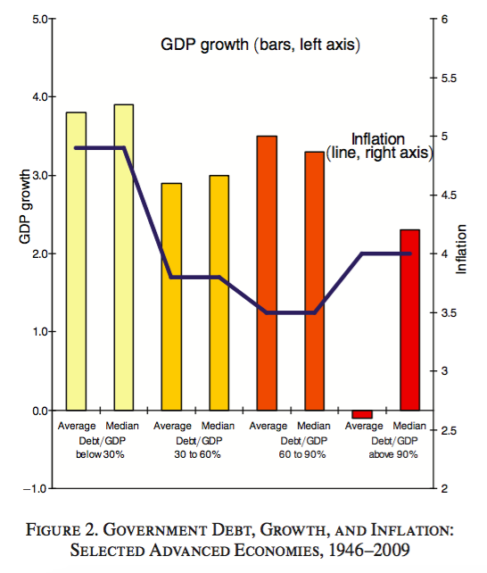
$The magical threshold of $90\%$ external debt.$

Figure 2.29: The magical threshold of $90\%$ external debt.

Herndon, Ash, and Pollin (2013) replicated the analysis of Reinhart and Rogoff (2010) and found that “selective exclusion of available data, coding errors and inappropriate weighting of summary statistics lead to serious miscalculations that inaccurately represent the relationship between public debt and GDP growth among 20 advanced economies.” The authors concluded that “both mean and median GDP growth when public debt levels exceed 90% of GDP are not dramatically different from when the public debt/GDP ratios are lower.” As a consequence, Reinhart and Rogoff (2010) led to an unjustified support for the adoption of austerity policies for countries with various levels of public debt.

You can read the full story at BBC, The New York Times and The Economist. Also, the video in Figure 2.30 contains a quick summary of the story by Nobel Prize laureate Paul Krugman.

Figure 2.30: CNN interview to Paul Krugman (key point from 1:16 to 1:40), broadcasted in 2013.

Herndon, Ash, and Pollin (2013) made the data of the study publicly available. You can download it here.

The dataset hap.txt (download) contains data for 20 advanced economies in the time period 1946–2009 and is the data source for the papers aforementioned. The variable dRGDP represents the real GDP growth (as a percentage) and debtgdp represents the percentage of public debt with respect to the GDP.

Import the data and save it as hap.
Set the case names of hap as Country.Year.
Summarize dRGDP and debtgdp. What are their minimum and maximum values?
What is the correlation between dRGDP and debtgdp? What is the standard deviation of each variable?
Show the scatterplot of dRGDP vs. debtgdp with the regression line. Is this coherent with what was stated in the video at 1:30?
Do you see any gap on the data around 90%? Is there any substantial change for dRGDP around there?
Compute the linear regression of dRGDP on debtgdp and summarize the fit.
What are the fitted coefficients? What are their standard errors? What is the $R^2$?
Compute the ANOVA table. How many degrees of freedom are? What is the SSR? What is SSE? What is the $p$-value for $H_0:\beta_1=0$?
Is SSR larger than SSE? Is this coherent with the resulting $R^2$?
Are $\beta_0$ and $\beta_1$ significant for the regression at level $\alpha=0.05$? And at level $\alpha=0.10,0.01$?
Compute the CIs for the coefficients. Can we conclude that the effect of debtgdp on dRGDP is positive at $\alpha=0.05$? And negative?
Predict the average growth for levels of debt of 60%, 70%, 80%, 90%, 100% and 110%. Compute the 95% CIs for all of them.
Predict the growth for the previous levels of debt. Compute also the CI for them. Is there a marked difference on the CIs for debt levels below and above 90%?
Which assumptions of the linear model you think are satisfied? Should we trust blindly the inferential results obtained assuming that the assumptions were satisfied?

References

Herndon, Thomas, Michael Ash, and Robert Pollin. 2013. “Does High Public Debt Consistently Stifle Economic Growth? A Critique of Reinhart and Rogoff.” Cambridge Journal of Economics. https://doi.org/10.1093/cje/bet075.

Moore, Gordon E. 1965. “Cramming More Components onto Integrated Circuits.” Electronics 38 (8): 114–17. https://doi.org/10.1109/JPROC.1998.658762.

Reinhart, Carmen M., and Kenneth S. Rogoff. 2010. “Growth in a Time of Debt.” Working Paper 15639. Working Paper Series. National Bureau of Economic Research. https://doi.org/10.3386/w15639.

The standardization of $X_1,\ldots,X_n$ is $Z_1,\ldots,Z_n$, with $Z_i=\frac{X_i-\bar X}{s_x}$, where $s_x$ is the standard deviation of $X_1,\ldots,X_n$.↩︎