3.6 ANOVA and model fit
3.6.1 ANOVA
The ANOVA decomposition for multiple linear regression is quite analogous to the one in simple linear regression. The ANOVA decomposes the variance of \(Y\) into two parts, each one corresponding to the regression and to the error, respectively. Since the difference between simple and multiple linear regression is the number of predictors – the response \(Y\) is unique in both cases – the ANOVA decompositions are highly similar, as we will see.
As in simple linear regression, the mean of the fitted values \(\hat Y_1,\ldots,\hat Y_n\) is the mean of \(Y_1,\ldots, Y_n\). This is an important result that can be checked if we use matrix notation. The ANOVA decomposition considers the following measures of variation related with the response:
- \(\text{SST}=\sum_{i=1}^n\left(Y_i-\bar Y\right)^2\), the total sum of squares. This is the total variation of \(Y_1,\ldots,Y_n\), since \(\text{SST}=ns_y^2\), where \(s_y^2\) is the sample variance of \(Y_1,\ldots,Y_n\).
- \(\text{SSR}=\sum_{i=1}^n\left(\hat Y_i-\bar Y\right)^2\), the regression sum of squares. This is the variation explained by the regression plane, that is, the variation from \(\bar Y\) that is explained by the estimated conditional mean \(\hat Y_i=\hat\beta_0+\hat\beta_1X_{i1}+\cdots+\hat\beta_kX_{ik}\). \(\text{SSR}=ns_{\hat y}^2\), where \(s_{\hat y}^2\) is the sample variance of \(\hat Y_1,\ldots,\hat Y_n\).
- \(\text{SSE}=\sum_{i=1}^n\left(Y_i-\hat Y_i\right)^2\), the sum of squared errors25. Is the variation around the conditional mean. Recall that \(\text{SSE}=\sum_{i=1}^n \hat\varepsilon_i^2=(n-k-1)\hat\sigma^2\), where \(\hat\sigma^2\) is the sample variance of \(\hat \varepsilon_1,\ldots,\hat \varepsilon_n\).
The ANOVA decomposition is exactly the same as in simple linear regression: \[\begin{align} \underbrace{\text{SST}}_{\text{Variation of }Y_i's} = \underbrace{\text{SSR}}_{\text{Variation of }\hat Y_i's} + \underbrace{\text{SSE}}_{\text{Variation of }\hat \varepsilon_i's} \tag{3.9} \end{align}\] or, equivalently (dividing by \(n\) in (3.9)), \[\begin{align*} \underbrace{s_y^2}_{\text{Variance of }Y_i's} = \underbrace{s_{\hat y}^2}_{\text{Variance of }\hat Y_i's} + \underbrace{(n-k-1)/n\times\hat\sigma^2}_{\text{Variance of }\hat\varepsilon_i's}. \end{align*}\] Notice the \(n-k-1\) instead of simple linear regression’s \(n-2\), which is the main change. The graphical interpretation of (3.9) when \(k=2\) is shown in Figures 3.11 and 3.12.
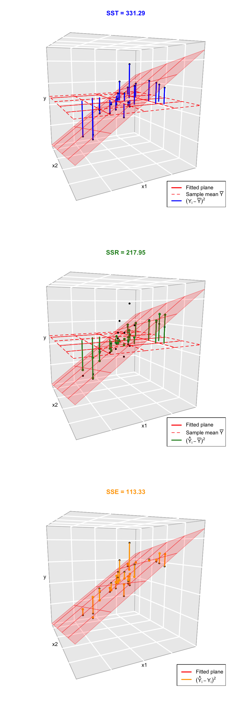
Figure 3.11: Visualization of the ANOVA decomposition when \(k=2\). SST measures the variation of \(Y_1,\ldots,Y_n\) with respect to \(\bar Y\). SST measures the variation with respect to the conditional means, \(\hat\beta_0+\hat\beta_1X_{i1}+\hat\beta_2X_{i2}\). SSE collects the variation of the residuals.
Figure 3.12: Illustration of the ANOVA decomposition and its dependence on \(\sigma^2\) and \(\hat\sigma^2\). Application also available here.
The ANOVA table summarizes the decomposition of the variance.
| Degrees of freedom | Sum Squares | Mean Squares | \(F\)-value | \(p\)-value | |
|---|---|---|---|---|---|
| Predictors | \(k\) | SSR | \(\frac{\text{SSR}}{k}\) | \(\frac{\text{SSR}/k}{\text{SSE}/(n-k-1)}\) | \(p\) |
| Residuals | \(n - k-1\) | SSE | \(\frac{\text{SSE}}{n-k-1}\) |
The “\(F\)-value” of the ANOVA table represents the value of the \(F\)-statistic \(\frac{\text{SSR}/k}{\text{SSE}/(n-k-1)}\). This statistic is employed to test \[\begin{align*} H_0:\beta_1=\ldots=\beta_k=0\quad\text{vs.}\quad H_1:\beta_j\neq 0\text{ for any }j, \end{align*}\] that is, the hypothesis of no linear dependence of \(Y\) on \(X_1,\ldots,X_k\) (the plane is completely flat, with no inclination). If \(H_0\) is rejected, it means that at least one \(\beta_j\) is significantly different from zero. It happens that \[\begin{align*} F=\frac{\text{SSR}/k}{\text{SSE}/(n-k-1)}\stackrel{H_0}{\sim} F_{k,n-k-1}, \end{align*}\] where \(F_{k,n-k-1}\) is the Snedecor’s \(F\) distribution with \(k\) and \(n-k-1\) degrees of freedom. If \(H_0\) is true, then \(F\) is expected to be small since SSR will be close to zero (little variation is explained by the regression model since \(\hat{\boldsymbol{\beta}}\approx\mathbf{0}\)). The \(p\)-value of this test is not the same as the \(p\)-value of the \(t\)-test for \(H_0:\beta_1=0\), that only happens in simple linear regression because \(k=1\)!
The “ANOVA table” is a broad concept in statistics, with different variants. Here we are only covering the basic ANOVA table from the relation \(\text{SST} = \text{SSR} + \text{SSE}\). However, further sophistications are possible when \(\text{SSR}\) is decomposed into the variations contributed by each predictor. In particular, for multiple linear regression R’s anova implements a sequential (type I) ANOVA table, which is not the previous table!
The anova function in R takes a model as an input and returns the following sequential ANOVA table26:
| Degrees of freedom | Sum Squares | Mean Squares | \(F\)-value | \(p\)-value | |
|---|---|---|---|---|---|
| Predictor 1 | \(1\) | SSR\(_1\) | \(\frac{\text{SSR}_1}{1}\) | \(\frac{\text{SSR}_1/1}{\text{SSE}/(n-k-1)}\) | \(p_1\) |
| Predictor 2 | \(1\) | SSR\(_2\) | \(\frac{\text{SSR}_2}{1}\) | \(\frac{\text{SSR}_2/1}{\text{SSE}/(n-k-1)}\) | \(p_2\) |
| \(\vdots\) | \(\vdots\) | \(\vdots\) | \(\vdots\) | \(\vdots\) | \(\vdots\) |
| Predictor \(k\) | \(1\) | SSR\(_k\) | \(\frac{\text{SSR}_k}{1}\) | \(\frac{\text{SSR}_k/1}{\text{SSE}/(n-k-1)}\) | \(p_k\) |
| Residuals | \(n - k - 1\) | SSE | \(\frac{\text{SSE}}{n-k-1}\) |
Here the SSR\(_j\) represents the regression sum of squares associated to the inclusion of \(X_j\) in the model with predictors \(X_1,\ldots,X_{j-1}\), this is: \[ \text{SSR}_j=\text{SSR}(X_1,\ldots,X_j)-\text{SSR}(X_1,\ldots,X_{j-1}). \] The \(p\)-values \(p_1,\ldots,p_k\) correspond to the testing of the hypotheses \[\begin{align*} H_0:\beta_j=0\quad\text{vs.}\quad H_1:\beta_j\neq 0, \end{align*}\] carried out inside the linear model \(Y=\beta_0+\beta_1X_1+\cdots+\beta_jX_j+\varepsilon\). This is like the \(t\)-test for \(\beta_j\) for the model with predictors \(X_1,\ldots,X_j\).
Let’s see how we can compute both ANOVA tables in R. The sequential table is simple: use anova. We illustrate it with the Boston dataset.
# Load data
library(MASS)
data(Boston)

# Fit a linear model
model <- lm(medv ~ crim + lstat + zn + nox, data = Boston)
summary(model)
##
## Call:
## lm(formula = medv ~ crim + lstat + zn + nox, data = Boston)
##
## Residuals:
##     Min      1Q  Median      3Q     Max
## -14.972  -3.956  -1.344   2.148  25.076
##
## Coefficients:
##             Estimate Std. Error t value Pr(>|t|)
## (Intercept) 30.93462    1.72076  17.977   <2e-16 ***
## crim        -0.08297    0.03677  -2.257   0.0245 *
## lstat       -0.90940    0.05040 -18.044   <2e-16 ***
## zn           0.03493    0.01395   2.504   0.0126 *
## nox          5.42234    3.24241   1.672   0.0951 .
## ---
## Signif. codes:  0 '***' 0.001 '**' 0.01 '*' 0.05 '.' 0.1 ' ' 1
##
## Residual standard error: 6.169 on 501 degrees of freedom
## Multiple R-squared:  0.5537, Adjusted R-squared:  0.5502
## F-statistic: 155.4 on 4 and 501 DF,  p-value: < 2.2e-16

# ANOVA table with sequential test
anova(model)
## Analysis of Variance Table
##
## Response: medv
##            Df  Sum Sq Mean Sq  F value  Pr(>F)
## crim        1  6440.8  6440.8 169.2694 < 2e-16 ***
## lstat       1 16950.1 16950.1 445.4628 < 2e-16 ***
## zn          1   155.7   155.7   4.0929 0.04360 *
## nox         1   106.4   106.4   2.7967 0.09509 .
## Residuals 501 19063.3    38.1
## ---
## Signif. codes:  0 '***' 0.001 '**' 0.01 '*' 0.05 '.' 0.1 ' ' 1
# The last p-value is the one of the last t-test
In order to compute the simplified ANOVA table, we need to rely on an ad-hoc function27. The function takes as input a fitted lm:
# This function computes the simplified anova from a linear model
simpleAnova <- function(object, ...) {

  # Compute anova table
  tab <- anova(object, ...)

  # Obtain number of predictors
  p <- nrow(tab) - 1

  # Add predictors row
  predictorsRow <- colSums(tab[1:p, 1:2])
  predictorsRow <- c(predictorsRow, predictorsRow[2] / predictorsRow[1])

  # F-quantities
  Fval <- predictorsRow[3] / tab[p + 1, 3]
  pval <- pf(Fval, df1 = p, df2 = tab$Df[p + 1], lower.tail = FALSE)
  predictorsRow <- c(predictorsRow, Fval, pval)

  # Simplified table
  tab <- rbind(predictorsRow, tab[p + 1, ])
  row.names(tab)[1] <- "Predictors"
  return(tab)

}

# Simplified ANOVA
simpleAnova(model)
## Analysis of Variance Table
##
## Response: medv
## Df Sum Sq Mean Sq F value Pr(>F)
## Predictors 4 23653 5913.3 155.41 < 2.2e-16 ***
## Residuals 501 19063 38.1
## ---
## Signif. codes: 0 '***' 0.001 '**' 0.01 '*' 0.05 '.' 0.1 ' ' 1Recall that the \(F\)-statistic, its \(p\)-value and the degrees of freedom are also given in the output of summary.
Compute the ANOVA table for the regression Price ~ WinterRain + AGST + HarvestRain + Age in the wine dataset. Check that the \(p\)-value for the \(F\)-test given in summary and by simpleAnova are the same.
3.6.2 The \(R^2\)
The coefficient of determination \(R^2\) is defined as in simple linear regression: \[\begin{align*} R^2=\frac{\text{SSR}}{\text{SST}}=\frac{\text{SSR}}{\text{SSR}+\text{SSE}}=\frac{\text{SSR}}{\text{SSR}+(n-k-1)\hat\sigma^2}. \end{align*}\] \(R^2\) measures the proportion of variation of the response variable \(Y\) that is explained by the predictors \(X_1,\ldots,X_k\) through the regression. Intuitively, \(R^2\) measures the tightness of the data cloud around the regression plane. Check in Figure 3.12 how changing the value of \(\sigma^2\) (not \(\hat\sigma^2\), but \(\hat\sigma^2\) is obviously dependent on \(\sigma^2\)) affects the \(R^2\). Also, as we saw in Section 2.7, \(R^2=r^2_{y\hat y}\), that is, the square of the sample correlation coefficient between \(Y_1,\ldots,Y_n\) and \(\hat Y_1,\ldots,\hat Y_n\) is \(R^2\).
Trusting blindly the \(R^2\) can lead to catastrophic conclusions in model selection. Here is a counterexample of a multiple regression where the \(R^2\) is apparently large but the assumptions discussed in Section 3.3 are clearly not satisfied.
# Create data that:
# 1) does not follow a linear model
# 2) the error is heteroskedastic
x1 <- seq(0.15, 1, l = 100)
set.seed(123456)
x2 <- runif(100, -3, 3)
eps <- rnorm(n = 100, sd = 0.25 * x1^2)
y <- 1 - 3 * x1 * (1 + 0.25 * sin(4 * pi * x1)) + 0.25 * cos(x2) + eps

# Great R^2!?
reg <- lm(y ~ x1 + x2)
summary(reg)
##
## Call:
## lm(formula = y ~ x1 + x2)
##
## Residuals:
##      Min       1Q   Median       3Q      Max
## -0.78737 -0.20946  0.01031  0.19652  1.05351
##
## Coefficients:
##              Estimate Std. Error t value Pr(>|t|)
## (Intercept)  0.788812   0.096418   8.181  1.1e-12 ***
## x1          -2.540073   0.154876 -16.401  < 2e-16 ***
## x2           0.002283   0.020954   0.109    0.913
## ---
## Signif. codes:  0 '***' 0.001 '**' 0.01 '*' 0.05 '.' 0.1 ' ' 1
##
## Residual standard error: 0.3754 on 97 degrees of freedom
## Multiple R-squared:  0.744,  Adjusted R-squared:  0.7388
## F-statistic:   141 on 2 and 97 DF,  p-value: < 2.2e-16
# But prediction is obviously problematic
scatter3d(y ~ x1 + x2, fit = "linear")Remember that:
- \(R^2\) does not measure the correctness of a linear model but its usefulness, assuming the model is correct.
- \(R^2\) is the proportion of variance of \(Y\) explained by \(X_1,\ldots,X_k\), but, of course, only when the linear model is correct.
We finalize by pointing out a nice connection between the \(R^2\), the ANOVA decomposition and the least squares estimator \(\hat{\boldsymbol{\beta}}\):
The ANOVA decomposition gives another interpretation of the least-squares estimates: \(\hat{\boldsymbol{\beta}}\) are the estimated coefficients that maximize the \(R^2\) (among all the possible estimates we could think about). To see this, recall that \[ R^2=\frac{\text{SSR}}{\text{SST}}=\frac{\text{SST} - \text{SSE}}{\text{SST}}=\frac{\text{SST} - \text{RSS}(\hat{\boldsymbol{\beta}})}{\text{SST}}, \] so if \(\text{RSS}(\hat{\boldsymbol{\beta}})=\min_{\boldsymbol{\beta}\in\mathbb{R}^{k+1}}\text{RSS}(\boldsymbol{\beta})\), then \(R^2\) is maximal for \(\hat{\boldsymbol{\beta}}\)!
3.6.3 The \(R^2_{\text{Adj}}\)
As we saw, these are equivalent forms for \(R^2\): \[\begin{align} R^2&=\frac{\text{SSR}}{\text{SST}}=\frac{\text{SST}-\text{SSE}}{\text{SST}}=1-\frac{\text{SSE}}{\text{SST}}\nonumber\\ &=1-\frac{\hat\sigma^2}{\text{SST}}\times(n-k-1).\tag{3.10} \end{align}\] The SSE on the numerator always decreases as more predictors are added to the model, even if these are no significant. As a consequence, the \(R^2\) always increases with \(k\). Why is so? Intuitively, because the complexity – hence the flexibility – of the model augments when we use more predictors to explain \(Y\). Mathematically, because when \(k\) approaches \(n-1\) the second term in (3.10) is reduced and, as a consequence, \(R^2\) grows.
The adjusted \(R^2\) is an important quantity specifically designed to cover this \(R^2\)’s flaw, which is ubiquitous in multiple linear regression. The purpose is to have a better tool for comparing models without systematically favoring complexer models. This alternative coefficient is defined as \[\begin{align} R^2_{\text{Adj}}&=1-\frac{\text{SSE}/(n-k-1)}{\text{SST}/(n-1)}=1-\frac{\text{SSE}}{\text{SST}}\times\frac{n-1}{n-k-1}\nonumber\\ &=1-\frac{\hat\sigma^2}{\text{SST}}\times (n-1).\tag{3.11} \end{align}\] The \(R^2_{\text{Adj}}\) is independent of \(k\), at least explicitly. If \(k=1\) then \(R^2_{\text{Adj}}\) is almost \(R^2\) (practically identical if \(n\) is large). Both (3.10) and (3.11) are quite similar except for the last factor, which in the former does not depend on \(k\). Therefore, (3.11) will only increase if \(\hat\sigma^2\) is reduced with \(k\) – in other words, if the new variables contribute in the reduction of variability around the regression plane.
The different behavior between \(R^2\) and \(R^2_\text{Adj}\) can be visualized by a small simulation. Suppose that we generate a random dataset, with \(n=200\) observations of a response \(Y\) and two predictors \(X_1,X_2\). This is, the sample \(\{(X_{i1},X_{i2},Y_i)\}_{i=1}^n\) with \[ Y_i=\beta_0+\beta_1X_{i1}+\beta_2X_{i2}+\varepsilon_i,\quad \varepsilon_i\sim\mathcal{N}(0,1). \] To this data, we add \(196\) garbage predictors that are completely independent from \(Y\). Therefore, we end up with \(k=198\) predictors. Now we compute the \(R^2(j)\) and \(R^2_\text{Adj}(j)\) for the models \[ Y=\beta_0+\beta_1X_{1}+\cdots+\beta_jX_{j}+\varepsilon, \] with \(j=1,\ldots,k\) and we plot them as the curves \((j,R^2(j))\) and \((j,R_\text{Adj}^2(j))\). Since \(R^2\) and \(R^2_\text{Adj}\) are random variables, we repeat the procedure \(100\) times to have a measure of the variability.
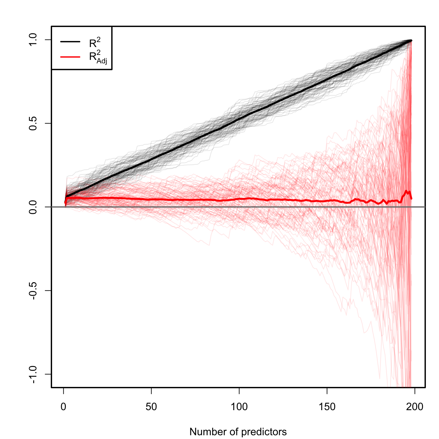
Figure 3.13: Comparison of \(R^2\) and \(R^2_{\text{Adj}}\) for \(n=200\) and \(k\) ranging from \(1\) to \(198\). \(M=100\) datasets were simulated with only the first two predictors being significant. The thicker curves are the mean of each color’s curves.
Figure 3.13 contains the results of this experiment. As you can see \(R^2\) increases linearly with the number of predictors considered, although only the first two ones were important! On the contrary, \(R^2_\text{Adj}\) only increases in the first two variables and then is flat on average, but it has a huge variability when \(k\) approaches \(n-2\). This is a consequence of the explosive variance of \(\hat\sigma^2\) in that degenerate case (as we will see in Section 3.7). The experiment evidences that \(R^2_\text{Adj}\) is more adequate than the \(R^2\) for evaluating the fit of a multiple linear regression.
An example of a simulated dataset considered in the experiment of Figure 3.13:
# Generate data
k <- 198
n <- 200
set.seed(3456732)
beta <- c(0.5, -0.5, rep(0, k - 2))
X <- matrix(rnorm(n * k), nrow = n, ncol = k)
Y <- drop(X %*% beta + rnorm(n, sd = 3))
data <- data.frame(y = Y, x = X)

# Regression on the two meaningful predictors
summary(lm(y ~ x.1 + x.2, data = data))

# Adding 20 garbage variables
summary(lm(y ~ X[, 1:22], data = data))
The \(R^2_\text{Adj}\) no longer measures the proportion of variation of \(Y\) explained by the regression, but the result of correcting this proportion by the number of predictors employed. As a consequence of this, \(R^2_\text{Adj}\leq1\) but it can be negative!
The next code illustrates a situation where we have two predictors completely independent from the response. The fitted model has a negative \(R^2_\text{Adj}\).
# Three independent variables
set.seed(234599)
x1 <- rnorm(100)
x2 <- rnorm(100)
y <- 1 + rnorm(100)

# Negative adjusted R^2
summary(lm(y ~ x1 + x2))
##
## Call:
## lm(formula = y ~ x1 + x2)
##
## Residuals:
##     Min      1Q  Median      3Q     Max
## -3.5081 -0.5021 -0.0191  0.5286  2.4750
##
## Coefficients:
##             Estimate Std. Error t value Pr(>|t|)
## (Intercept)  0.97024    0.10399   9.330 3.75e-15 ***
## x1           0.09003    0.10300   0.874    0.384
## x2          -0.05253    0.11090  -0.474    0.637
## ---
## Signif. codes:  0 '***' 0.001 '**' 0.01 '*' 0.05 '.' 0.1 ' ' 1
##
## Residual standard error: 1.034 on 97 degrees of freedom
## Multiple R-squared:  0.009797,   Adjusted R-squared:  -0.01062
## F-statistic: 0.4799 on 2 and 97 DF,  p-value: 0.6203
Construct more predictors (x3, x4, …) by sampling 100 points from a normal (rnorm(100)). Check that when the predictors are added to the model, the \(R^2_\text{Adj}\) decreases and the \(R^2\) increases.
SSE and RSS are two names for the same quantity (that appears in different contexts): \(\text{SSE}=\sum_{i=1}^n\left(Y_i-\hat Y_i\right)^2=\sum_{i=1}^n\left(Y_i-\hat \beta_0-\hat \beta_1X_{i1}-\cdots-\hat \beta_kX_{ik}\right)^2=\mathrm{RSS}(\hat{\boldsymbol{\beta}})\).↩︎
More complex – included here just for clarification of the
anova’s output.↩︎You will need to run this piece of code whenever you want to call
simpleAnova, since it is not part of R nor R Commander.↩︎