3.2 Model formulation and estimation by least squares

The multiple linear model extends the simple linear model by describing the relation between the random variables $X_1,\ldots,X_k$ and $Y$. For example, in the last model for the wine dataset, we had $k=4$ variables $X_1=$WinterRain, $X_2=$AGST, $X_3=$HarvestRain and $X_4=$Age and $Y=$ Price. Therefore, as in Section 2.3, the multiple linear model is constructed by assuming that the linear relation $$\begin{align} Y = \beta_0 + \beta_1 X_1 + \cdots + \beta_k X_k + \varepsilon \tag{3.1} \end{align}$$ holds between the predictors $X_1,\ldots,X_k$ and the response $Y$. In (3.1), $\beta_0$ is the intercept and $\beta_1,\ldots,\beta_k$ are the slopes, respectively. $\varepsilon$ is a random variable with mean zero and independent from $X_1,\ldots,X_k$. Another way of looking at (3.1) is $$\begin{align} \mathbb{E}[Y|X_1=x_1,\ldots,X_k=x_k]=\beta_0+\beta_1x_1+\cdots+\beta_kx_k, \tag{3.2} \end{align}$$ since $\mathbb{E}[\varepsilon|X_1=x_1,\ldots,X_k=x_k]=0$.

The LHS of (3.2) is the conditional expectation of $Y$ given $X_1,\ldots,X_k$. It represents how the mean of the random variable $Y$ is changing according to particular values, denoted by $x_1,\ldots,x_k$, of the random variables $X_1,\ldots,X_k$. With the RHS, what we are saying is that the mean of $Y$ is changing in a linear fashion with respect to the values of $X_1,\ldots,X_k$. Hence the interpretation of the coefficients:

• $\beta_0$: is the mean of $Y$ when $X_1=\ldots=X_k=0$.
• $\beta_j$, $1\leq j\leq k$: is the increment in mean of $Y$ for an increment of one unit in $X_j=x_j$, provided that the remaining variables $X_1,\ldots,X_{j-1},X_{j+1},\ldots,X_k$ do not change.

Figure 3.5 illustrates the geometrical interpretation of a multiple linear model: a plane in the $(k+1)$-dimensional space. If $k=1$, the plane is the regression line for simple linear regression. If $k=2$, then the plane can be visualized in a three-dimensional plot

Figure 3.5: The least squares regression plane $y=\hat\beta_0+\hat\beta_1x_1+\hat\beta_2x_2$ and its dependence on the kind of squared distance considered. Application also available here.

The estimation of $\beta_0,\beta_1,\ldots,\beta_k$ is done as in simple linear regression, by minimizing the Residual Sum of Squares (RSS). First we need to introduce some helpful matrix notation. In the following, bold face are used for distinguishing vectors and matrices from scalars:

• A sample of $(X_1,\ldots,X_k,Y)$ is $(X_{11},\ldots,X_{1k},Y_1),\ldots,(X_{n1},\ldots,X_{nk},Y_n)$, where $X_{ij}$ denotes the $i$-th observation of the $j$-th predictor $X_j$. We denote with $\mathbf{X}_i=(X_{i1},\ldots,X_{ik})$ to the $i$-th observation of $(X_1,\ldots,X_k)$, so the sample simplifies to $(\mathbf{X}_{1},Y_1),\ldots,(\mathbf{X}_{n},Y_n)$.

• The design matrix contains all the information of the predictors and a column of ones $$\mathbf{X}=\begin{pmatrix} 1 & X_{11} & \cdots & X_{1k}\\ \vdots & \vdots & \ddots & \vdots\\ 1 & X_{n1} & \cdots & X_{nk} \end{pmatrix}_{n\times(k+1)}.$$

• The vector of responses $\mathbf{Y}$, the vector of coefficients $\boldsymbol{\beta}$ and the vector of errors are, respectively²², $$\mathbf{Y}=\begin{pmatrix} Y_1 \\ \vdots \\ Y_n \end{pmatrix}_{n\times 1},\quad\boldsymbol{\beta}=\begin{pmatrix} \beta_0 \\ \beta_1 \\ \vdots \\ \beta_k \end{pmatrix}_{(k+1)\times 1}\text{ and } \boldsymbol{\varepsilon}=\begin{pmatrix} \varepsilon_1 \\ \vdots \\ \varepsilon_n \end{pmatrix}_{n\times 1}.$$ Thanks to the matrix notation, we can turn the sample version of the multiple linear model, namely $$Y_i=\beta_0 + \beta_1 X_{i1} + \cdots +\beta_k X_{ik} + \varepsilon_i,\quad i=1,\ldots,n,$$ into something as compact as $$\mathbf{Y}=\mathbf{X}\boldsymbol{\beta}+\boldsymbol{\varepsilon}.$$

Recall that if $k=1$ we have the simple linear model. In this case: $$\mathbf{X}=\begin{pmatrix} 1 & X_{11}\\ \vdots & \vdots\\ 1 & X_{n1} \end{pmatrix}_{n\times2}\text{ and } \beta=\begin{pmatrix} \beta_0 \\ \beta_1 \end{pmatrix}_{2\times 1}.$$

The RSS for the multiple linear regression is $$\begin{align} \text{RSS}(\boldsymbol{\beta})&=\sum_{i=1}^n(Y_i-\beta_0-\beta_1X_{i1}-\cdots-\beta_kX_{ik})^2\nonumber\\ &=(\mathbf{Y}-\mathbf{X}\boldsymbol{\beta})^T(\mathbf{Y}-\mathbf{X}\boldsymbol{\beta}).\tag{3.3} \end{align}$$ The RSS aggregates the squared vertical distances from the data to a regression plane given by $\boldsymbol{\beta}$. Remember that the vertical distances are considered because we want to minimize the error in the prediction of $Y$. The least squares estimators are the minimizers of the RSS²³: $$\begin{align*} \hat{\boldsymbol{\beta}}=\arg\min_{\boldsymbol{\beta}\in\mathbb{R}^{k+1}} \text{RSS}(\boldsymbol{\beta}). \end{align*}$$ Luckily, thanks to the matrix form of (3.3), it is simple to compute a closed-form expression for the least squares estimates: $$\begin{align} \hat{\boldsymbol{\beta}}=(\mathbf{X}^T\mathbf{X})^{-1}\mathbf{X}^T\mathbf{Y}.\tag{3.4} \end{align}$$

There are some similarities between (3.4) and $\hat\beta_1=(s_x^2)^{-1}s_{xy}$ from the simple linear model: both are related to the covariance between $\mathbf{X}$ and $Y$ weighted by the variance of $\mathbf{X}$.

The data of the illustration has been generated with the following code:

# Generates 50 points from a N(0, 1): predictors and error
set.seed(34567) # Fixes the seed for the random generator
x1 <- rnorm(50)
x2 <- rnorm(50)
x3 <- x1 + rnorm(50, sd = 0.05) # Make variables dependent
eps <- rnorm(50)

# Responses
yLin <- -0.5 + 0.5 * x1 + 0.5 * x2 + eps
yQua <- -0.5 + x1^2 + 0.5 * x2 + eps
yExp <- -0.5 + 0.5 * exp(x2) + x3 + eps

# Data
leastSquares3D <- data.frame(x1 = x1, x2 = x2, yLin = yLin,
                             yQua = yQua, yExp = yExp)

Let’s check that indeed the coefficients given by lm are the ones given by equation (3.4) for the regression yLin ~ x1 + x2.

# Matrix X
X <- cbind(1, x1, x2)

# Vector Y
Y <- yLin

# Coefficients
beta <- solve(t(X) %*% X) %*% t(X) %*% Y
# %*% multiplies matrices
# solve() computes the inverse of a matrix
# t() transposes a matrix
beta
##          [,1]
##    -0.5702694
## x1  0.4832624
## x2  0.3214894

# Output from lm
mod <- lm(yLin ~ x1 + x2, data = leastSquares3D)
mod$coefficients
## (Intercept)          x1          x2 
##  -0.5702694   0.4832624   0.3214894

Compute $\boldsymbol{\beta}$ for the regressions yLin ~ x1 + x2, yQua ~ x1 + x2 and yExp ~ x2 + x3 using:

• equation (3.4) and
• the function lm.

Check that the fitted plane and the coefficient estimates are coherent.

Once we have the least squares estimates $\hat{\boldsymbol{\beta}}$, we can define the next two concepts:

• The fitted values $\hat Y_1,\ldots,\hat Y_n$, where $$\begin{align*} \hat Y_i=\hat\beta_0+\hat\beta_1X_{i1}+\cdots+\hat\beta_kX_{ik},\quad i=1,\ldots,n. \end{align*}$$ They are the vertical projections of $Y_1,\ldots,Y_n$ into the fitted line (see Figure 3.5). In a matrix form, inputting (3.3) $$\hat{\mathbf{Y}}=\mathbf{X}\hat{\boldsymbol{\beta}}=\mathbf{X}(\mathbf{X}^T\mathbf{X})^{-1}\mathbf{X}^T\mathbf{Y}=\mathbf{H}\mathbf{Y},$$ where $\mathbf{H}=\mathbf{X}(\mathbf{X}^T\mathbf{X})^{-1}\mathbf{X}^T$ is called the hat matrix because it “puts the hat into $\mathbf{Y}$.” What it does is to project $\mathbf{Y}$ into the regression plane (see Figure 3.5).

• The residuals (or estimated errors) $\hat \varepsilon_1,\ldots,\hat \varepsilon_n$, where $$\begin{align*} \hat\varepsilon_i=Y_i-\hat Y_i,\quad i=1,\ldots,n. \end{align*}$$ They are the vertical distances between actual data and fitted data.

We conclude with an insight on the relation of multiple and simple linear regressions. It is illustrated in Figure 3.6.

Consider the multiple linear model $Y=\beta_0+\beta_1X_1+\beta_2X_2+\varepsilon$ and its associated simple linear models $Y=\alpha_0+\alpha_1X_1+\varepsilon$ and $Y=\gamma_0+\gamma_1X_2+\varepsilon$. Assume that we have a sample $(X_{11},X_{12},Y_1),\ldots, (X_{n1},X_{n2},Y_n)$. Then, in general, $\hat\alpha_0\neq\hat\beta_0$, $\hat\alpha_1\neq\hat\beta_1$, $\hat\gamma_0\neq\hat\beta_0$ and $\hat\gamma_1\neq\hat\beta_1$. This is, in general, the inclusion of a new predictor changes the coefficient estimates.

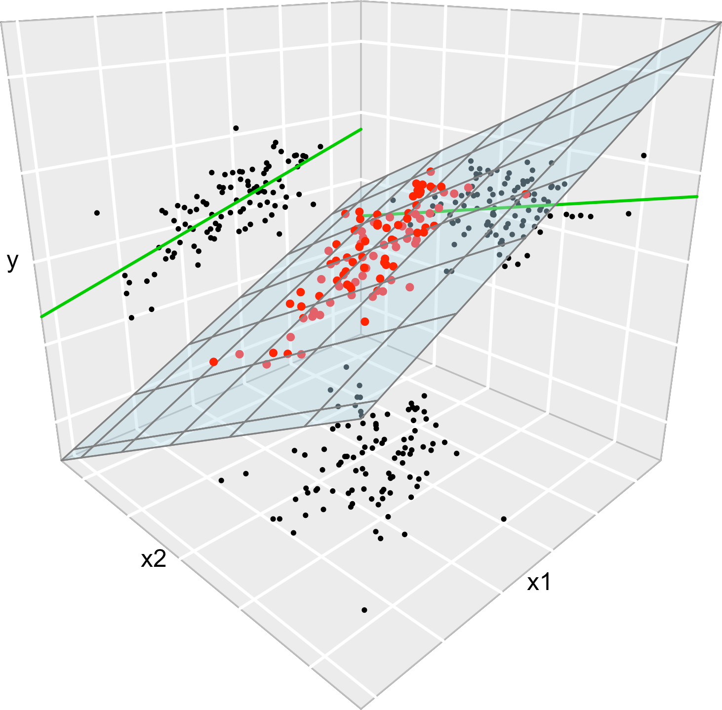
Figure 3.6: The regression plane (blue) and its relation with the simple linear regressions (green lines). The red points represent the sample for $(X_1,X_2,Y)$ and the black points the subsamples for $(X_1,X_2)$ (bottom), $(X_1,Y)$ (left) and $(X_2,Y)$ (right).

The data employed in Figure 3.6 is:

set.seed(212542)
n <- 100
x1 <- rnorm(n, sd = 2)
x2 <- rnorm(n, mean = x1, sd = 3)
y <- 1 + 2 * x1 - x2 + rnorm(n, sd = 1)
data <- data.frame(x1 = x1, x2 = x2, y = y)

With the above data, check how the fitted coefficients change for y ~ x1, y ~ x2 and y ~ x1 + x2.

---

22. The vectors are regarded as column matrices.↩︎

23. They are unique and always exist.↩︎