2.5 Inference for the model coefficients

The assumptions introduced in the previous section allow to specify what is the distribution of the random variables $\hat\beta_0$ and $\hat\beta_1$. As we will see, this is a key point for making inference on $\beta_0$ and $\beta_1$.

The distributions are derived conditionally on the sample predictors $X_1,\ldots,X_n$. In other words, we assume that the randomness of $Y_i=\beta_0+\beta_1X_i+\varepsilon_i$, $i=1,\ldots,n$, comes only from the error terms and not from the predictors. To denote this, we employ lowercase for the sample predictors $x_1,\ldots,x_n$.

2.5.1 Distributions of the fitted coefficients

The distributions of $\hat\beta_0$ and $\hat\beta_1$ are: $$\begin{align} \hat\beta_0\sim\mathcal{N}\left(\beta_0,\mathrm{SE}(\hat\beta_0)^2\right),\quad\hat\beta_1\sim\mathcal{N}\left(\beta_1,\mathrm{SE}(\hat\beta_1)^2\right)\tag{2.4} \end{align}$$ where $$\begin{align} \mathrm{SE}(\hat\beta_0)^2=\frac{\sigma^2}{n}\left[1+\frac{\bar X^2}{s_x^2}\right],\quad \mathrm{SE}(\hat\beta_1)^2=\frac{\sigma^2}{ns_x^2}.\tag{2.5} \end{align}$$ Recall that an equivalent form for (2.4) is (why?) $$\begin{align*} \frac{\hat\beta_0-\beta_0}{\mathrm{SE}(\hat\beta_0)}\sim\mathcal{N}(0,1),\quad\frac{\hat\beta_1-\beta_1}{\mathrm{SE}(\hat\beta_1)}\sim\mathcal{N}(0,1). \end{align*}$$

Some important remarks on (2.4) and (2.5) are

• Bias. Both estimates are unbiased. That means that their expectations are the true coefficients.

• Variance. The variances $\mathrm{SE}(\hat\beta_0)^2$ and $\mathrm{SE}(\hat\beta_1)^2$ have an interesting interpretation in terms of its components:

  • Sample size $n$. As the sample size grows, the precision of the estimators increases, since both variances decrease.

  • Error variance $\sigma^2$. The more disperse the error is, the less precise the estimates are, since the more vertical variability is present.

  • Predictor variance $s_x^2$. If the predictor is spread out (large $s_x^2$), then it is easier to fit a regression line: we have information about the data trend over a long interval. If $s_x^2$ is small, then all the data is concentrated on a narrow vertical band, so we have a much more limited view of the trend.

  • Mean $\bar X$. It has influence only on the precision of $\hat\beta_0$. The larger $\bar X$ is, the less precise $\hat\beta_0$ is.

Figure 2.20: Illustration of the randomness of the fitted coefficients $(\hat\beta_0,\hat\beta_1)$ and the influence of $n$, $\sigma^2$ and $s_x^2$. The sample predictors $x_1,\ldots,x_n$ are fixed and new responses $Y_1,\ldots,Y_n$ are generated each time from a linear model $Y=\beta_0+\beta_1X+\varepsilon$. Application also available here.

The problem with (2.4) and (2.5) is that $\sigma^2$ is unknown in practice, so we need to estimate $\sigma^2$ from the data. We do so by computing the sample variance of the residuals $\hat\varepsilon_1,\ldots,\hat\varepsilon_n$. First note that the residuals have zero mean. This can be easily seen by replacing $\hat\beta_0=\bar Y-\hat\beta_1\bar X$: $$\begin{align} \bar\varepsilon =\frac{1}{n}\sum_{i=1}^n(Y_i-\hat\beta_0-\hat\beta_1X_i)=\frac{1}{n}\sum_{i=1}^n(Y_i-\bar Y+\hat\beta_1\bar X-\hat\beta_1X_i)=0. \end{align}$$ Due to this, we can and we can do it by computing a rescaled sample variance of the residuals: $$\begin{align*} \hat\sigma^2=\frac{\sum_{i=1}^n\hat\varepsilon_i^2}{n-2}. \end{align*}$$ Note the $n-2$ in the denominator, instead of $n$! $n-2$ are the degrees of freedom and is the number of data points minus the number of already fitted parameters. The interpretation is that “we have consumed $2$ degrees of freedom of the sample on fitting $\hat\beta_0$ and $\hat\beta_1$.”

If we use the estimate $\hat\sigma^2$ instead of $\sigma^2$, we get different – and more useful – distributions for $\beta_0$ and $\beta_1$: $$\begin{align} \frac{\hat\beta_0-\beta_0}{\hat{\mathrm{SE}}(\hat\beta_0)}\sim t_{n-2},\quad\frac{\hat\beta_1-\beta_1}{\hat{\mathrm{SE}}(\hat\beta_1)}\sim t_{n-2}\tag{2.6} \end{align}$$ where $t_{n-2}$ represents the Student’s $t$ distribution¹⁰ with $n-2$ degrees of freedom and $$\begin{align} \hat{\mathrm{SE}}(\hat\beta_0)^2=\frac{\hat\sigma^2}{n}\left[1+\frac{\bar X^2}{s_x^2}\right],\quad \hat{\mathrm{SE}}(\hat\beta_1)^2=\frac{\hat\sigma^2}{ns_x^2}\tag{2.7} \end{align}$$ are the estimates of $\mathrm{SE}(\hat\beta_0)^2$ and $\mathrm{SE}(\hat\beta_1)^2$. The LHS of (2.6) is called the $t$-statistic because of its distribution. The interpretation of (2.7) is analogous to the one of (2.5).

2.5.2 Confidence intervals for the coefficients

Due to (2.6) and (2.7), we can have the $100(1-\alpha)\%$ Confidence Intervals (CI) for the coefficients: $$\begin{align} \left(\hat\beta_j\pm\hat{\mathrm{SE}}(\hat\beta_j)t_{n-2;\alpha/2}\right),\quad j=0,1,\tag{2.8} \end{align}$$ where $t_{n-2;\alpha/2}$ is the $\alpha/2$-upper quantile of the $t_{n-2}$ (see Figure 2.21). Usually, $\alpha=0.10,0.05,0.01$ are considered.

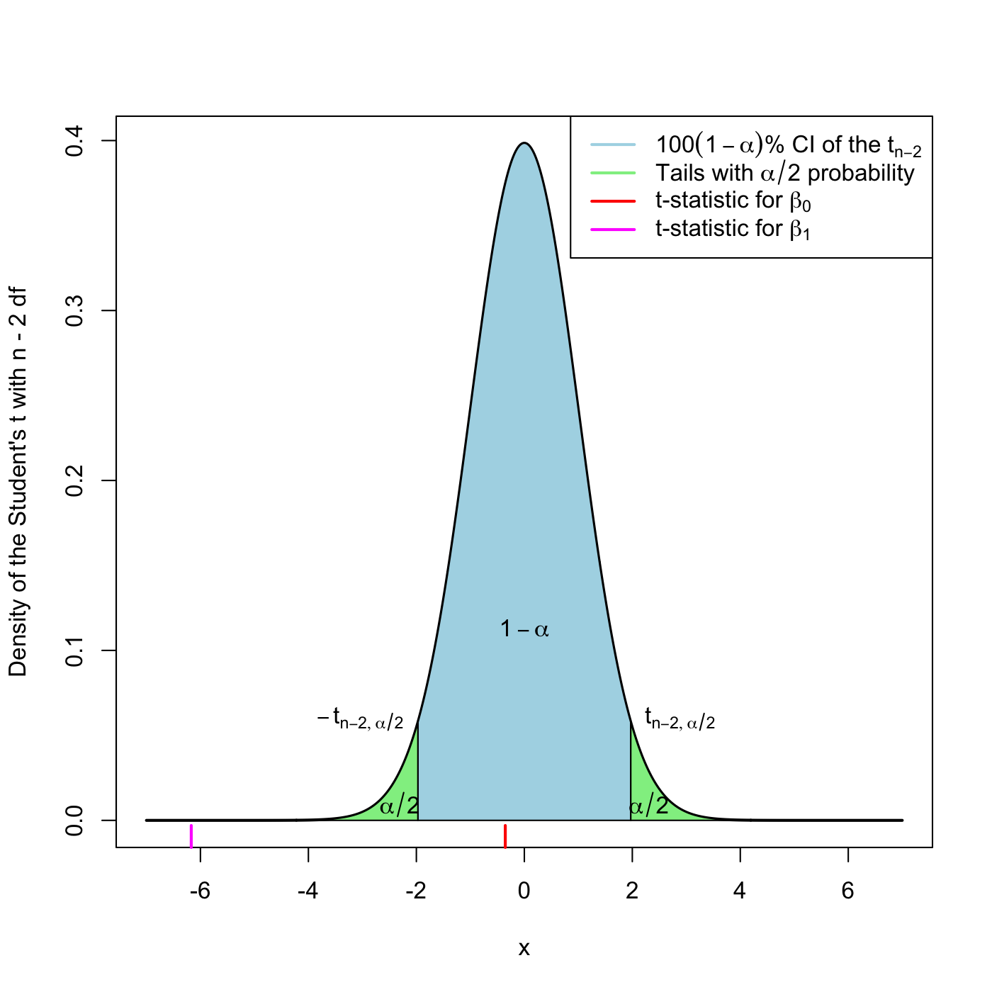
Figure 2.21: The Student’s $t$ distribution for the $t$-statistics associated to null intercept and slope, for the y1 ~ x1 regression of the assumptions dataset.

Do you need to remember the above equations? No, although you need to fully understand them. R + R Commander will compute everything for you through the functions lm, summary and confint.

This random CI contains the unknown coefficient $\beta_j$ with a probability of $1-\alpha$. Note also that the CI is symmetric around $\hat\beta_j$. A simple way of understanding this concept is as follows. Suppose you have 100 samples generated according to a linear model. If you compute the CI for a coefficient, then in approximately $100(1-\alpha)$ of the samples the true coefficient would be actually inside the random CI. This is illustrated in Figure 2.22.

Figure 2.22: Illustration of the randomness of the CI for $\beta_0$ at $100(1-\alpha)\%$ confidence. The plot shows 100 random CIs for $\beta_0$, computed from 100 random datasets generated by the same linear model, with intercept $\beta_0$. The illustration for $\beta_1$ is completely analogous. Application also available here.

Let’s see how we can compute the CIs for $\beta_0$ and $\beta_1$ in practice. We do it in the first regression of the assumptions dataset. Assuming you have loaded the dataset, in R we can simply type:

mod1 <- lm(y1 ~ x1, data = assumptions)
confint(mod1)
##                  2.5 %     97.5 %
## (Intercept) -0.2256901  0.1572392
## x1          -0.5587490 -0.2881032

In this example, the 95% confidence interval for $\beta_0$ is $(-0.2257, 0.1572)$. For $\beta_1$ is $(-0.5587, -0.2881)$. Therefore, we can say that with a 95% confidence x1 has a negative effect on y1. If the CI for $\beta_1$ was $(-0.2256901, 0.1572392)$, we could not arrive to the same conclusion, since the CI contains both positive and negative numbers.

By default, the confidence interval is computed for $\alpha=0.05$. You can change this on the level argument, for example:

confint(mod1, level = 0.90) # alpha = 0.10
##                    5 %       95 %
## (Intercept) -0.1946762  0.1262254
## x1          -0.5368291 -0.3100231
confint(mod1, level = 0.95) # alpha = 0.05
##                  2.5 %     97.5 %
## (Intercept) -0.2256901  0.1572392
## x1          -0.5587490 -0.2881032
confint(mod1, level = 0.99) # alpha = 0.01
##                  0.5 %     99.5 %
## (Intercept) -0.2867475  0.2182967
## x1          -0.6019030 -0.2449492

Note that the larger the confidence of the interval, the longer – thus less useful – it is. For example, the interval $(-\infty,\infty)$ contains any coefficient with a 100% confidence, but is completely useless.

If you want to make the CIs through the help of R Commander (assuming the dataset has been loaded and is the active one), then do the following:

1. Fit the linear model ('Statistics' -> 'Fit models' -> 'Linear regression...').
2. Go to 'Models' -> 'Confidence intervals...' and then input the 'Condifence Level'.

Compute the CIs (95%) for the coefficients of the regressions:

• y2 ~ x2
• y6 ~ x6
• y7 ~ x7

Do you think all of them are meaningful? Which ones are and why? (Recall: inference on the model makes sense if assumptions of the model are verified)

Compute the CIs for the coefficients of the following regressions:

• MathMean ~ ScienceMean (pisa)
• MathMean ~ ReadingMean (pisa)
• Seats2013.2023 ~ Population2010 (US)
• CamCom2011 ~ Population2010 (EU)

For the above regressions, can we conclude with a 95% confidence that the effect of the predictor is positive in the response?

A CI for $\sigma^2$ can be also computed, but is less important in practice. The formula is: $$\begin{align*} \left(\frac{n-2}{\chi^2_{n-2;\alpha/2}}\hat\sigma^2,\frac{n-2}{\chi^2_{n-2;1-\alpha/2}}\hat\sigma^2\right) \end{align*}$$ where $\chi^2_{n-2;q}$ is the $q$-upper quantile of the $\chi^2$ distribution¹¹ with $n-2$ degrees of freedom, $\chi^2_{n-2}$. Note that the CI is not symmetric around $\hat\sigma^2$.

Compute the CI for $\sigma^2$ for the regression of MathMean on logGDPp in the pisa dataset. Do it for $\alpha=0.10,0.05,0.01$.

• To compute $\chi^2_{n-2;q}$, you can do:

  • In R by qchisq(p = q, df = n - 2, lower.tail = FALSE).
  • In R Commander, go to ‘Distributions’ -> ‘Continuous distributions’ -> ‘Chi-squared distribution’ -> ‘Chi-squared quantiles’ and then select ‘Upper tail’. Input $q$ as the ‘Probabilities’ and $n-2$ as the ‘Degrees of freedom’.

• To compute $\hat\sigma^2$, use summary(lm(MathMean ~ logGDPp, data = pisa))$sigma^2. Remember that there are 65 countries in the study.

Answers: c(1720.669, 3104.512), c(1635.441, 3306.257) and c(1484.639, 3752.946).

2.5.3 Testing on the coefficients

The distributions in (2.6) also allow to conduct a formal hypothesis test on the coefficients $\beta_j$, $j=0,1$. For example the test for significance (shortcut for significantly difference from zero) is specially important, that is, the test of the hypotheses $$\begin{align*} H_0:\beta_j=0 \end{align*}$$ for $j=0,1$. The test of $H_0:\beta_1=0$ is specially interesting, since it allows to answer whether the variable $X$ has a significant linear effect on $Y$. The statistic used for testing for significance is the $t$-statistic $$\begin{align*} \frac{\hat\beta_j-0}{\hat{\mathrm{SE}}(\hat\beta_j)}, \end{align*}$$ which is distributed as a $t_{n-2}$ under the (veracity of) the null hypothesis.

Remember the analogy of hypothesis testing vs a trial, as given in the table below.

Hypothesis testing	Trial
Null hypothesis $H_0$	Accused of committing a crime. It has the “presumption of innocence,” which means that it is not guilty until there is enough evidence to supporting its guilt
Sample $X_1,\ldots,X_n$	Collection of small evidences supporting innocence and guilt
Statistic $T_n$	Summary of the evidence presented by the prosecutor and defense lawyer
Distribution of $T_n$ under $H_0$	The judge conducting the trial. Evaluates the evidence presented by both sides and presents a verdict for $H_0$
Significance level $\alpha$	$1-\alpha$ is the strength of evidences required by the judge for condemning $H_0$. The judge allows evidences that on average condemn $100\alpha\%$ of the innocents! $\alpha=0.05$ is considered a reasonable level
$p$-value	Decision of the judge. If $p\text{-value}<\alpha$, $H_0$ is declared guilty. Otherwise, is declared not guilty
$H_0$ is rejected	$H_0$ is declared guilty: there are strong evidences supporting its guilt
$H_0$ is not rejected	$H_0$ is declared not guilty: either is innocent or there are no enough evidences supporting its guilt

More formally, the $p$-value is defined as:

The $p$-value is the probability of obtaining a statistic more unfavourable to $H_0$ than the observed, assuming that $H_0$ is true.

Therefore, if the $p$-value is small (smaller than the chosen level $\alpha$), it is unlikely that the evidence against $H_0$ is due to randomness. As a consequence, $H_0$ is rejected. If the $p$-value is large (larger than $\alpha$), then it is more possible that the evidences against $H_0$ are merely due to the randomness of the data. In this case, we do not reject $H_0$.

The null hypothesis $H_0$ is tested against the alternative hypothesis, $H_1$. If $H_0$ is rejected, it is rejected in favor of $H_1$. The alternative hypothesis can be bilateral, such as $$\begin{align*} H_0:\beta_j= 0\quad\text{vs}\quad H_1:\beta_j\neq 0 \end{align*}$$ or unilateral, such as $$\begin{align*} H_0:\beta_j\geq (\leq)0\quad\text{vs}\quad H_1:\beta_j<(>)0 \end{align*}$$ For the moment, we will focus only on the bilateral case.

The connection of a $t$-test for $H_0:\beta_j=0$ and the CI for $\beta_j$, both at level $\alpha$, is the following.

Is $0$ inside the CI for $\beta_j$?

• Yes $\leftrightarrow$ do not reject $H_0$.
• No $\leftrightarrow$ reject $H_0$.

The tests for significance are built-in in the summary function, as we glimpsed in Section 2.1.2. For mod1, we have:

summary(mod1)
## 
## Call:
## lm(formula = y1 ~ x1, data = assumptions)
## 
## Residuals:
##      Min       1Q   Median       3Q      Max 
## -2.13678 -0.62218 -0.07824  0.54671  2.63056 
## 
## Coefficients:
##             Estimate Std. Error t value Pr(>|t|)    
## (Intercept) -0.03423    0.09709  -0.353    0.725    
## x1          -0.42343    0.06862  -6.170 3.77e-09 ***
## ---
## Signif. codes:  0 '***' 0.001 '**' 0.01 '*' 0.05 '.' 0.1 ' ' 1
## 
## Residual standard error: 0.9559 on 198 degrees of freedom
## Multiple R-squared:  0.1613, Adjusted R-squared:  0.157 
## F-statistic: 38.07 on 1 and 198 DF,  p-value: 3.772e-09

The Coefficients block of the output of summary contains the next elements regarding the test $H_0:\beta_j=0$ vs $H_1:\beta_j\neq0$:

• Estimate: least squares estimate $\hat\beta_j$.
• Std. Error: estimated standard error $\hat{\mathrm{SE}}(\hat\beta_j)$.
• t value: $t$-statistic $\frac{\hat\beta_j}{\hat{\mathrm{SE}}(\hat\beta_j)}$.
• Pr(>|t|): $p$-value of the $t$-test.
• Signif. codes: 0 '***' 0.001 '**' 0.01 '*' 0.05 '.' 0.1 ' ' 1: codes indicating the size of the $p$-value. The more stars, the more evidence supporting that $H_0$ does not hold.

In the above output for summary(mod1), $H_0:\beta_0=0$ is not rejected at any reasonable level for $\alpha$ (that is, $0.10$,$0.05$ and $0.01$). Hence $\hat\beta_0$ is not significantly different from zero and $\beta_0$ is not significant for the regression. On the other hand, $H_0:\beta_1=0$ is rejected at any level $\alpha$ larger than the $p$-value, 3.77e-09. Therefore, $\beta_1$ is significant for the regression (and $\hat\beta_1$ is not significantly different from zero).

For the assumptions dataset, do the next:

• Regression y7 ~ x7. Check that:
  • The intercept of is not significant for the regression at any reasonable level $\alpha$.
  • The slope is significant for any $\alpha\geq 10^{-7}$.
• Regression y6 ~ x6. Assume the linear model assumptions are verified.
  • Check that $\hat\beta_0$ is significantly different from zero at any level $\alpha$.
  • For which $\alpha=0.10,0.05,0.01$ is $\hat\beta_1$ significantly different from zero?

Re-analyze the significance of the coefficients in Seats2013.2023 ~ Population2010 and Seats2011 ~ Population2010 for the US and EU datasets, respectively.

---

10. The Student’s $t$ distribution has heavier tails than the normal, which means that large observations in absolute value are more likely. $t_n$ converges to a $\mathcal{N}(0,1)$ when $n$ is large. For example, with $n$ larger than $30$, the normal is a good approximation.↩︎

11. $\chi_n^2$ is the distribution of the sum of the squares of $n$ random variables $\mathcal{N}(0,1)$.↩︎