3.7 Model selection
In Section 3.1.1 we briefly saw that the inclusion of more predictors is not for free: there is a price to pay in terms of more variability on the coefficients. Indeed, there is a maximum number of predictors \(k\) that can be considered in a linear model for a sample size \(n\): \(k\leq n-2\). Or equivalently, there is a minimum sample size \(n\) required for fitting a model with \(k\) predictors: \(n\geq k + 2\).
The interpretation of this fact is simple if we think on the geometry for \(k=1\) and \(k=2\):
- If \(k=1\), we need at least \(n=2\) points to fit uniquely a line. However, this line gives no information on the vertical variation around it and hence \(\hat\sigma^2\) can not be estimated (applying its formula, we would have \(\hat\sigma^2=\infty\)). Therefore we need at least \(n=3\) points, or in other words \(n\geq k + 2=3\).
- If \(k=2\), we need at least \(n=3\) points to fit uniquely a plane. But this plane gives no information on the variation of the data around it and hence \(\hat\sigma^2\) can not be estimated. Therefore we need \(n\geq k + 2=4\).
Another interpretation is the following:
The fitting of a linear model with \(k\) predictors involves the estimation the \(k+2\) parameters \((\boldsymbol{\beta},\sigma^2)\) from \(n\) data points. The closer \(k+2\) and \(n\) are, the more variable the estimates \((\hat{\boldsymbol{\beta}},\hat\sigma^2)\) will be, since less information is available for estimating each one. In the limit case \(n=k+2\), each sample point determines a parameter estimate.
The degrees of freedom \(n-k-1\) quantify the increasing on the variability of \((\hat{\boldsymbol{\beta}},\hat\sigma^2)\) when \(n-k-1\) decreases. For example:
- \(t_{n-k-1;\alpha/2}\) appears in (3.7) and influences the length of the CIs for \(\beta_j\), see (3.8). It also influences the length of the CIs for the prediction. As Figure 3.14 shows, when the degrees of freedom decrease, \(t_{n-k-1;\alpha/2}\) increases, thus the intervals become wider.
- \(\hat\sigma^2=\frac{1}{n-k-1}\sum_{i=1}^n\hat\varepsilon_i^2\) influences the \(R^2\) and \(R^2_\text{Adj}\). If no relevant variables are added to the model then \(\sum_{i=1}^n\hat\varepsilon_i^2\) will not change substantially. However, the reducing factor \(\frac{1}{n-k-1}\) will decrease as \(k\) augments, inflating \(\hat\sigma^2\) and its variance. This is exactly what happened in Figure 3.13.
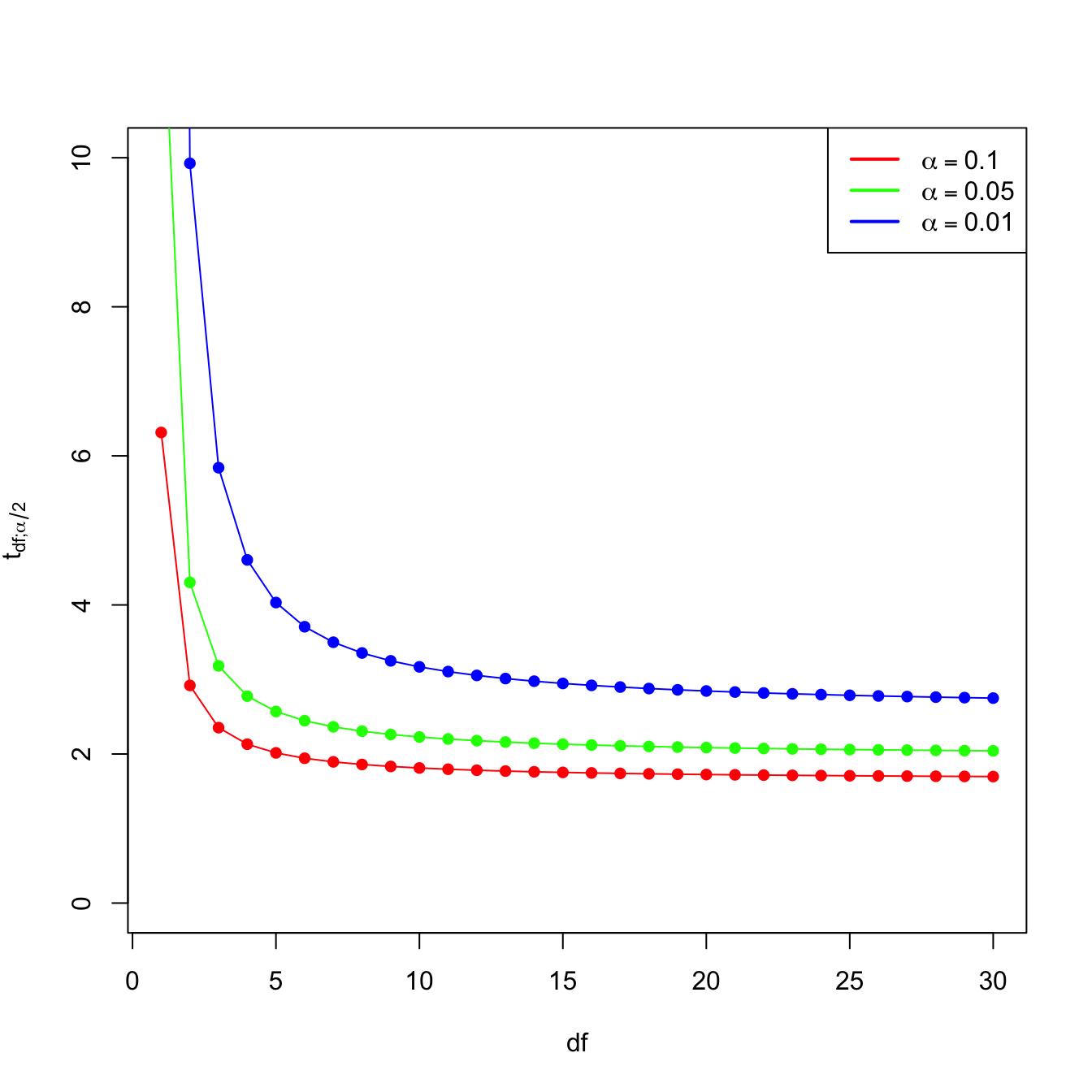
Figure 3.14: Effect of \(\text{df}=n-k-1\) in \(t_{\text{df};\alpha/2}\) for \(\alpha=0.10,0.05,0.01\).
Now that we have added more light into the problem of having an excess of predictors, we turn the focus into selecting the most adequate predictors for a multiple regression model. This is a challenging task without a unique solution, and what is worse, without a method that is guaranteed to work in all the cases. However, there is a well-established procedure that usually gives good results: the stepwise regression. Its principle is to compare multiple linear regression models with different predictors (and, of course, with the same responses).
Before introducing the method, we need to understand what is an information criterion. An information criterion balances the fitness of a model with the number of predictors employed. Hence, it determines objectively the best model as the one that minimizes the information criterion. Two common criteria are the Bayesian Information Criterion (BIC) and the Akaike Information Criterion (AIC). Both are based on a balance between the model fitness and its complexity: \[\begin{align} \text{BIC}(\text{model}) = \underbrace{-2\log\text{lik(model)}}_{\text{Model fitness}} + \underbrace{\text{npar(model)}\times\log n}_{\text{Complexity}}, \tag{3.12} \end{align}\] where \(\text{lik(model)}\) is the likelihood of the model (how well the model fits the data) and \(\text{npar(model)}\) is the number of parameters of the model, \(k+2\) in the case of a multiple linear regression model with \(k\) predictors. The AIC replaces \(\log n\) by \(2\) in (3.12), so it penalizes less complexer models. This is one of the reasons why BIC is preferred by some practitioners for model comparison. Also, because is consistent in selecting the true model: if enough data is provided, the BIC is guaranteed to select the data-generating model among a list of candidate models.
The BIC and AIC can be computed in R through the functions BIC and AIC. They take a model as the input.
# Load iris dataset
data(iris)

# Two models with different predictors
mod1 <- lm(Petal.Length ~ Sepal.Width, data = iris)
mod2 <- lm(Petal.Length ~ Sepal.Width + Petal.Width, data = iris)

# BICs
BIC(mod1)
## [1] 579.7856
BIC(mod2) # Smaller -> better
## [1] 208.0366

# Check the summaries
summary(mod1)
##
## Call:
## lm(formula = Petal.Length ~ Sepal.Width, data = iris)
##
## Residuals:
##     Min      1Q  Median      3Q     Max
## -3.7721 -1.4164  0.1719  1.2094  4.2307
##
## Coefficients:
##             Estimate Std. Error t value Pr(>|t|)
## (Intercept)   9.0632     0.9289   9.757  < 2e-16 ***
## Sepal.Width  -1.7352     0.3008  -5.768 4.51e-08 ***
## ---
## Signif. codes:  0 '***' 0.001 '**' 0.01 '*' 0.05 '.' 0.1 ' ' 1
##
## Residual standard error: 1.6 on 148 degrees of freedom
## Multiple R-squared:  0.1836, Adjusted R-squared:  0.178
## F-statistic: 33.28 on 1 and 148 DF,  p-value: 4.513e-08
summary(mod2)
##
## Call:
## lm(formula = Petal.Length ~ Sepal.Width + Petal.Width, data = iris)
##
## Residuals:
##      Min       1Q   Median       3Q      Max
## -1.33753 -0.29251 -0.00989  0.21447  1.24707
##
## Coefficients:
##             Estimate Std. Error t value Pr(>|t|)
## (Intercept)  2.25816    0.31352   7.203 2.84e-11 ***
## Sepal.Width -0.35503    0.09239  -3.843  0.00018 ***
## Petal.Width  2.15561    0.05283  40.804  < 2e-16 ***
## ---
## Signif. codes:  0 '***' 0.001 '**' 0.01 '*' 0.05 '.' 0.1 ' ' 1
##
## Residual standard error: 0.4574 on 147 degrees of freedom
## Multiple R-squared:  0.9338, Adjusted R-squared:  0.9329
## F-statistic:  1036 on 2 and 147 DF,  p-value: < 2.2e-16
Let’s go back to the selection of predictors. If we have \(k\) predictors, a naive procedure would be to check all the possible models that can be constructed with them and then select the best one in terms of BIC/AIC. The problem is that there are \(2^{k+1}\) possible models! Fortunately, the stepwise procedure helps us navigating this ocean of models. The function takes as input a model employing all the available predictors.
# Explain NOx in Boston dataset
mod <- lm(nox ~ ., data = Boston)

# With BIC
modBIC <- stepwise(mod, trace = 0)
##
## Direction:  backward/forward
## Criterion:  BIC
summary(modBIC)
##
## Call:
## lm(formula = nox ~ indus + age + dis + rad + ptratio + medv,
##     data = Boston)
##
## Residuals:
##       Min        1Q    Median        3Q       Max
## -0.117146 -0.034877 -0.005863  0.031655  0.183363
##
## Coefficients:
##               Estimate Std. Error t value Pr(>|t|)
## (Intercept)  0.7649531  0.0347425  22.018  < 2e-16 ***
## indus        0.0045930  0.0005972   7.691 7.85e-14 ***
## age          0.0008682  0.0001381   6.288 7.03e-10 ***
## dis         -0.0170889  0.0020226  -8.449 3.24e-16 ***
## rad          0.0033154  0.0003730   8.888  < 2e-16 ***
## ptratio     -0.0130209  0.0013942  -9.339  < 2e-16 ***
## medv        -0.0021057  0.0003413  -6.170 1.41e-09 ***
## ---
## Signif. codes:  0 '***' 0.001 '**' 0.01 '*' 0.05 '.' 0.1 ' ' 1
##
## Residual standard error: 0.05485 on 499 degrees of freedom
## Multiple R-squared:  0.7786, Adjusted R-squared:  0.7759
## F-statistic: 292.4 on 6 and 499 DF,  p-value: < 2.2e-16

# Different search directions
stepwise(mod, trace = 0, direction = "forward")
##
## Direction:  forward
## Criterion:  BIC
##
## Call:
## lm(formula = nox ~ dis + indus + age + rad + ptratio + medv,
##     data = Boston)
##
## Coefficients:
## (Intercept)          dis        indus          age          rad      ptratio
##   0.7649531   -0.0170889    0.0045930    0.0008682    0.0033154   -0.0130209
##        medv
##  -0.0021057
stepwise(mod, trace = 0, direction = "backward")
##
## Direction:  backward
## Criterion:  BIC
##
## Call:
## lm(formula = nox ~ indus + age + dis + rad + ptratio + medv,
##     data = Boston)
##
## Coefficients:
## (Intercept)        indus          age          dis          rad      ptratio
##   0.7649531    0.0045930    0.0008682   -0.0170889    0.0033154   -0.0130209
##        medv
##  -0.0021057

# With AIC
modAIC <- stepwise(mod, trace = 0, criterion = "AIC")
##
## Direction:  backward/forward
## Criterion:  AIC
summary(modAIC)
##
## Call:
## lm(formula = nox ~ crim + indus + age + dis + rad + ptratio +
##     medv, data = Boston)
##
## Residuals:
##       Min        1Q    Median        3Q       Max
## -0.122633 -0.035593 -0.004273  0.030938  0.182914
##
## Coefficients:
##               Estimate Std. Error t value Pr(>|t|)
## (Intercept)  0.7750308  0.0349903  22.150  < 2e-16 ***
## crim        -0.0007603  0.0003753  -2.026   0.0433 *
## indus        0.0044875  0.0005976   7.509 2.77e-13 ***
## age          0.0008656  0.0001377   6.288 7.04e-10 ***
## dis         -0.0175329  0.0020282  -8.645  < 2e-16 ***
## rad          0.0037478  0.0004288   8.741  < 2e-16 ***
## ptratio     -0.0132746  0.0013956  -9.512  < 2e-16 ***
## medv        -0.0022716  0.0003499  -6.491 2.06e-10 ***
## ---
## Signif. codes:  0 '***' 0.001 '**' 0.01 '*' 0.05 '.' 0.1 ' ' 1
##
## Residual standard error: 0.05468 on 498 degrees of freedom
## Multiple R-squared:  0.7804, Adjusted R-squared:  0.7773
## F-statistic: 252.8 on 7 and 498 DF,  p-value: < 2.2e-16
The model selected by stepwise is a good starting point for further additions or deletions of predictors. For example, in modAIC we could remove crim.
When applying stepwise for BIC/AIC, different final models might be selected depending on the choice of direction. This is the interpretation:
-
“backward”: starts from the full model, removes predictors sequentially. -
“forward”: starts from the simplest model, adds predictors sequentially. -
“backward/forward”(default) and“forward/backward”: combination of the above.
The advice is to try several of these methods and retain the one with minimum BIC/AIC. Set trace = 0 to omit lengthy outputs of information of the search procedure.
stepwise assumes that no NA’s (missing values) are present in the data. It is advised to remove the missing values in the data before since their presence might lead to errors. To do so, employ data = na.omit(dataset) in the call to lm (if your dataset is dataset).
We conclude highlighting a caveat on the use of the BIC and AIC: they are constructed assuming that the sample size \(n\) is much larger than the number of parameters in the model (\(k+2\)). Therefore, they will work reasonably well if \(n>>k+2\), but if this is not true they may favor unrealistic complex models. An illustration of this phenomena is Figure 3.15, which is the BIC/AIC version of Figure 3.13 for the experiment done in Section 3.6. The BIC and AIC curves tend to have local minimums close to \(k=2\) and then increase. But when \(k+2\) gets close to \(n\), they quickly drop down. Note also how the BIC penalizes more the complexity than the AIC, which is more flat.
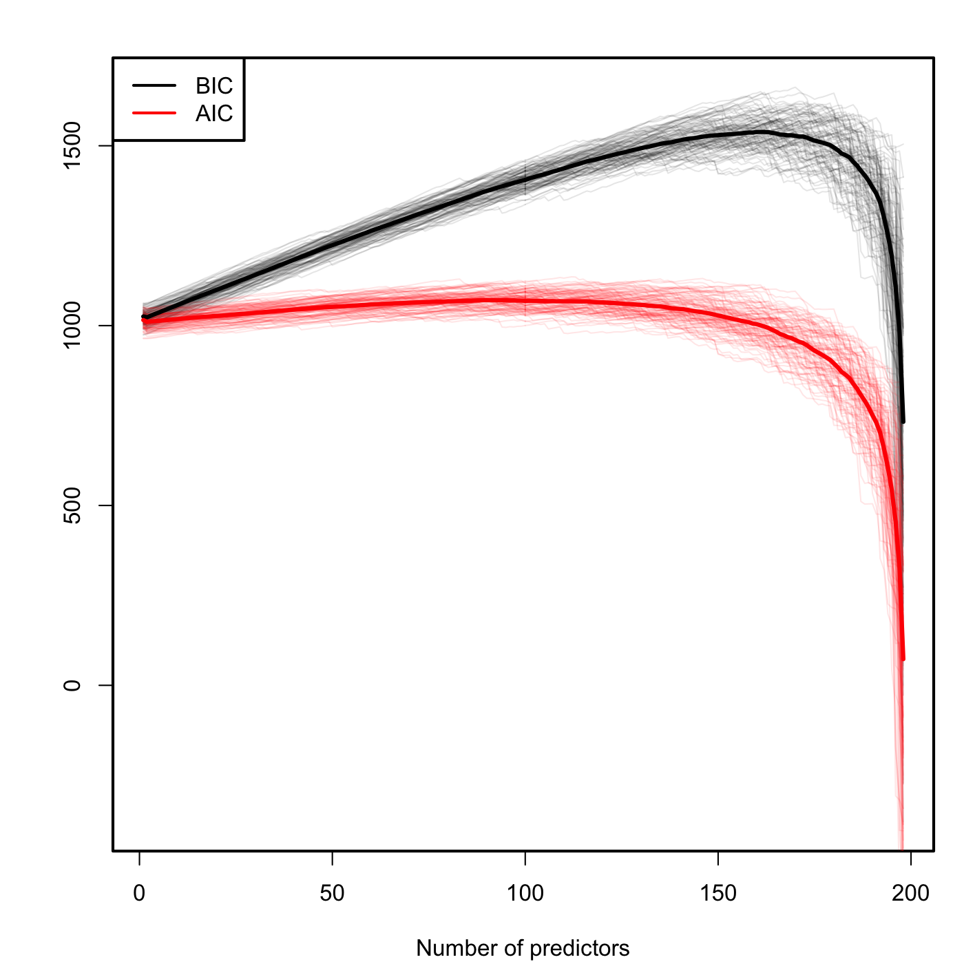
Figure 3.15: Comparison of BIC and AIC for \(n=200\) and \(k\) ranging from \(1\) to \(198\). \(M=100\) datasets were simulated with only the first two predictors being significant. The thicker curves are the mean of each color’s curves.