3.1 Examples and applications
3.1.1 Case study I: The Bordeaux equation
Calculate the winter rain and the harvest rain (in millimeters). Add summer heat in the vineyard (in degrees centigrade). Subtract 12.145. And what do you have? A very, very passionate argument over wine.
— “Wine Equation Puts Some Noses Out of Joint,” The New York Times, 04/03/1990
This case study is motivated by the study of Princeton professor Orley Ashenfelter (Ashenfelter, Ashmore, and Lalonde 1995) on the quality of red Bordeaux vintages. The study became mainstream after disputes with the wine press, especially with Robert Parker, Jr., one of the most influential wine critic in America. See a short review of the story at the Financial Times (Google’s cache) and at the video in Figure 3.3.
Red Bordeaux wines have been produced in Bordeaux, one of most famous and prolific wine regions in the world, in a very similar way for hundreds of years. However, the quality of vintages is largely variable from one season to another due to a long list of random factors, such as the weather conditions. Because Bordeaux wines taste better when they are older (young wines are astringent, when the wines age they lose their astringency), there is an incentive to store the young wines until they are mature. Due to the important difference in taste, it is hard to determine the quality of the wine when it is so young just by tasting it, because it is going to change substantially when the aged wine is in the market. Therefore, being able to predict the quality of a vintage is a valuable information for investing resources, for determining a fair price for vintages and for understanding what factors are affecting the wine quality. The purpose of this case study is to answer:
- Q1. Can we predict the quality of a vintage effectively?
- Q2. What is the interpretation of such prediction?
The wine.csv file (download) contains 27 red Bordeaux vintages. The data is the originally employed by Ashenfelter, Ashmore, and Lalonde (1995), except for the inclusion of the variable Year, the exclusion of NAs and the reference price used for the wine. The original source is here. Each row has the following variables:
Year: year in which grapes were harvested to make wine.Price: logarithm of the average market price for Bordeaux vintages according to 1990–1991 auctions.17 This is a nonlinear transformation of the response (hence different to what we did in Section 2.8) made to linearize the response.WinterRain: winter rainfall (in mm).AGST: Average Growing Season Temperature (in Celsius degrees).HarvestRain: harvest rainfall (in mm).Age: age of the wine measured as the number of years stored in a cask.FrancePop: population of France atYear(in thousands).
The quality of the wine is quantified as the Price, a clever way of quantifying a qualitative measure. The data is shown in Table 3.1.
| Year | Price | WinterRain | AGST | HarvestRain | Age | FrancePop |
|---|---|---|---|---|---|---|
| 1952 | 7.4950 | 600 | 17.1167 | 160 | 31 | 43183.57 |
| 1953 | 8.0393 | 690 | 16.7333 | 80 | 30 | 43495.03 |
| 1955 | 7.6858 | 502 | 17.1500 | 130 | 28 | 44217.86 |
| 1957 | 6.9845 | 420 | 16.1333 | 110 | 26 | 45152.25 |
| 1958 | 6.7772 | 582 | 16.4167 | 187 | 25 | 45653.81 |
| 1959 | 8.0757 | 485 | 17.4833 | 187 | 24 | 46128.64 |
| 1960 | 6.5188 | 763 | 16.4167 | 290 | 23 | 46584.00 |
| 1961 | 8.4937 | 830 | 17.3333 | 38 | 22 | 47128.00 |
| 1962 | 7.3880 | 697 | 16.3000 | 52 | 21 | 48088.67 |
| 1963 | 6.7127 | 608 | 15.7167 | 155 | 20 | 48798.99 |
| 1964 | 7.3094 | 402 | 17.2667 | 96 | 19 | 49356.94 |
| 1965 | 6.2518 | 602 | 15.3667 | 267 | 18 | 49801.82 |
| 1966 | 7.7443 | 819 | 16.5333 | 86 | 17 | 50254.97 |
| 1967 | 6.8398 | 714 | 16.2333 | 118 | 16 | 50650.41 |
| 1968 | 6.2435 | 610 | 16.2000 | 292 | 15 | 51034.41 |
Let’s begin by summarizing the information in Table 3.1. First, import correctly the dataset into R Commander and 'Set case names...' as the variable Year. Let’s summarize and inspect the data in two ways:
Numerically. Go to
'Statistics' -> 'Summaries' -> 'Active data set'.summary(wine) ## Price WinterRain AGST HarvestRain ## Min. :6.205 Min. :376.0 Min. :14.98 Min. : 38.0 ## 1st Qu.:6.508 1st Qu.:543.5 1st Qu.:16.15 1st Qu.: 88.0 ## Median :6.984 Median :600.0 Median :16.42 Median :123.0 ## Mean :7.042 Mean :608.4 Mean :16.48 Mean :144.8 ## 3rd Qu.:7.441 3rd Qu.:705.5 3rd Qu.:17.01 3rd Qu.:185.5 ## Max. :8.494 Max. :830.0 Max. :17.65 Max. :292.0 ## Age FrancePop ## Min. : 3.00 Min. :43184 ## 1st Qu.: 9.50 1st Qu.:46856 ## Median :16.00 Median :50650 ## Mean :16.19 Mean :50085 ## 3rd Qu.:22.50 3rd Qu.:53511 ## Max. :31.00 Max. :55110Additionally, other summary statistics are available in
'Statistics' -> 'Summaries' -> 'Numerical summaries...'.Graphically. Make a scatterplot matrix with all the variables. Add the
'Least-squares lines','Histograms'on the diagonals and choose to identify 2 points.scatterplotMatrix(~ Age + AGST + FrancePop + HarvestRain + Price + WinterRain, reg.line = lm, smooth = FALSE, spread = FALSE, span = 0.5, ellipse = FALSE, levels = c(.5, .9), id.n = 2, diagonal = 'histogram', data = wine)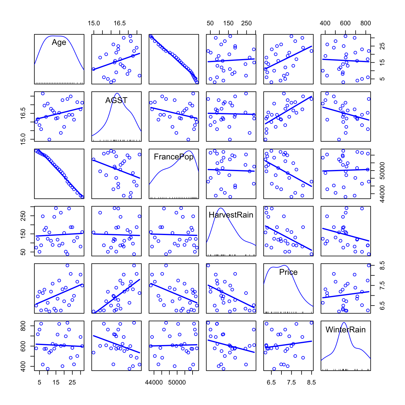
Figure 3.1: Scatterplot matrix for
wine.
Recall that the objective is to predict Price. Based on the above matrix scatterplot the best we can predict Price by a simple linear regression seems to be with AGST or HarvestRain. Let’s see which one yields the larger \(R^2\).
modAGST <- lm(Price ~ AGST, data = wine)
summary(modAGST)
##
## Call:
## lm(formula = Price ~ AGST, data = wine)
##
## Residuals:
##      Min       1Q   Median       3Q      Max
## -0.78370 -0.23827 -0.03421  0.29973  0.90198
##
## Coefficients:
##             Estimate Std. Error t value Pr(>|t|)
## (Intercept)  -3.5469     2.3641  -1.500 0.146052
## AGST          0.6426     0.1434   4.483 0.000143 ***
## ---
## Signif. codes:  0 '***' 0.001 '**' 0.01 '*' 0.05 '.' 0.1 ' ' 1
##
## Residual standard error: 0.4819 on 25 degrees of freedom
## Multiple R-squared:  0.4456, Adjusted R-squared:  0.4234
## F-statistic: 20.09 on 1 and 25 DF,  p-value: 0.0001425

modHarvestRain <- lm(Price ~ HarvestRain, data = wine)
summary(modHarvestRain)
##
## Call:
## lm(formula = Price ~ HarvestRain, data = wine)
##
## Residuals:
##      Min       1Q   Median       3Q      Max
## -1.03792 -0.27679 -0.07892  0.40434  1.21958
##
## Coefficients:
##              Estimate Std. Error t value Pr(>|t|)
## (Intercept)  7.679856   0.241911  31.747  < 2e-16 ***
## HarvestRain -0.004405   0.001497  -2.942  0.00693 **
## ---
## Signif. codes:  0 '***' 0.001 '**' 0.01 '*' 0.05 '.' 0.1 ' ' 1
##
## Residual standard error: 0.5577 on 25 degrees of freedom
## Multiple R-squared:  0.2572, Adjusted R-squared:  0.2275
## F-statistic: 8.658 on 1 and 25 DF,  p-value: 0.00693
In Price ~ AGST, the intercept is not significant for the regression but the slope is, and AGST has a positive effect on the Price. For Price ~ HarvestRain, both intercept and slope are significant and the effect is negative.
Complete the analysis by computing the linear models Price ~ FrancePop, Price ~ Age and Price ~ WinterRain. Name them as modFrancePop, modAge and modWinterRain. Check if the intercepts and slopes are significant for the regression.
If we do the simple regressions of Price on the remaining predictors, we obtain a table like this for the \(R^2\):
| Predictor | \(R^2\) |
|---|---|
AGST |
\(0.4456\) |
HarvestRain |
\(0.2572\) |
FrancePop |
\(0.2314\) |
Age |
\(0.2120\) |
WinterRain |
\(0.0181\) |
A natural question to ask is:
Can we combine these simple regressions to increase both the \(R^2\) and the prediction accuracy for
Price?
The answer is yes, by means of the multiple linear regression. In order to make our first one, go to 'Statistics' -> 'Fit models' -> 'Linear model...'. A window like Figure 3.2 will pop-up.
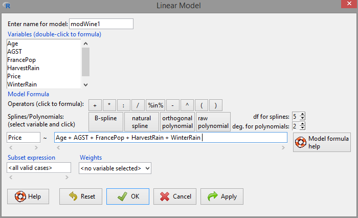
Figure 3.2: Window for performing multiple linear regression.
Set the response as Price and add the rest of variables as predictors, in the form Age + AGST + FrancePop + HarvestRain + WinterRain. Note the use of + for including all the predictors. This does not mean that they are all summed and then the regression is done on the sum!18. Instead of, this notation is designed to resemble the multiple linear model:
\[\begin{align*}
Y=\beta_0+\beta_1X_1+\beta_2X_2+\cdots+\beta_kX_k+\varepsilon
\end{align*}\]
If the model is named modWine1, we get the following summary when clicking in 'OK':
modWine1 <- lm(Price ~ Age + AGST + FrancePop + HarvestRain + WinterRain, data = wine)
summary(modWine1)
##
## Call:
## lm(formula = Price ~ Age + AGST + FrancePop + HarvestRain + WinterRain,
##     data = wine)
##
## Residuals:
##      Min       1Q   Median       3Q      Max
## -0.46541 -0.24133  0.00413  0.18974  0.52495
##
## Coefficients:
##               Estimate Std. Error t value Pr(>|t|)
## (Intercept) -2.343e+00  7.697e+00  -0.304  0.76384
## Age          1.377e-02  5.821e-02   0.237  0.81531
## AGST         6.144e-01  9.799e-02   6.270 3.22e-06 ***
## FrancePop   -2.213e-05  1.268e-04  -0.175  0.86313
## HarvestRain -3.837e-03  8.366e-04  -4.587  0.00016 ***
## WinterRain   1.153e-03  4.991e-04   2.311  0.03109 *
## ---
## Signif. codes:  0 '***' 0.001 '**' 0.01 '*' 0.05 '.' 0.1 ' ' 1
##
## Residual standard error: 0.293 on 21 degrees of freedom
## Multiple R-squared:  0.8278, Adjusted R-squared:  0.7868
## F-statistic: 20.19 on 5 and 21 DF,  p-value: 2.232e-07
The main difference with simple linear regressions is that we have more rows on the 'Coefficients' section, since these correspond to each of the predictors. The fitted regression is Price \(= -2.343 + 0.013\,\times\) Age \(+ 0.614\,\times\) AGST \(- 0.000\,\times\) FrancePop \(- 0.003\,\times\) HarvestRain \(+ 0.001\,\times\) WinterRain
. Recall that the 'Multiple R-squared' has almost doubled with respect to the best simple linear regression!19 This tells us that we can explain up to \(82.75\%\) of the Price variability by the predictors.
Note however that many predictors are not significant for the regression: FrancePop, Age and the intercept are not significant. This is an indication of an excess of predictors adding little information to the response. Note the almost perfect correlation between FrancePop and Age shown in Figure 3.1: one of them is not adding any extra information to explain Price. This complicates the model unnecessarily and, more importantly, it has the undesirable effect of making the coefficient estimates less precise. We opt to remove the predictor FrancePop from the model since it is exogenous to the wine context.
Two useful tips about lm’s syntax for including/excluding predictors faster:
-
Price ~ .-> includes all the variables in the dataset as predictors. It is equivalent toPrice ~ Age + AGST + FrancePop + HarvestRain + WinterRain. -
Price ~ . - FrancePop-> includes all the variables except the ones with-as predictors. It is equivalent to It is equivalent toPrice ~ Age + AGST + HarvestRain + WinterRain.
Then, the model without FrancePop is
modWine2 <- lm(Price ~ . - FrancePop, data = wine)
summary(modWine2)
##
## Call:
## lm(formula = Price ~ . - FrancePop, data = wine)
##
## Residuals:
##      Min       1Q   Median       3Q      Max
## -0.46024 -0.23862  0.01347  0.18601  0.53443
##
## Coefficients:
##               Estimate Std. Error t value Pr(>|t|)
## (Intercept) -3.6515703  1.6880876  -2.163  0.04167 *
## WinterRain   0.0011667  0.0004820   2.420  0.02421 *
## AGST         0.6163916  0.0951747   6.476 1.63e-06 ***
## HarvestRain -0.0038606  0.0008075  -4.781 8.97e-05 ***
## Age          0.0238480  0.0071667   3.328  0.00305 **
## ---
## Signif. codes:  0 '***' 0.001 '**' 0.01 '*' 0.05 '.' 0.1 ' ' 1
##
## Residual standard error: 0.2865 on 22 degrees of freedom
## Multiple R-squared:  0.8275, Adjusted R-squared:  0.7962
## F-statistic: 26.39 on 4 and 22 DF,  p-value: 4.057e-08
All the coefficients are significant at level \(\alpha=0.05\). Therefore, there is no clear redundant information. In addition, the \(R^2\) is very similar to the full model, but the 'Adjusted R-squared', a weighting of the \(R^2\) to account for the number of predictors used by the model, is slightly larger. Hence, this means that, comparatively to the number of predictors used, modWine2 explains more variability of Price than modWine1. Later in this chapter we will see the precise meaning of the \(R^2\) adjusted.
The comparison of the coefficients of both models can be done with 'Models -> Compare model coefficients...':
compareCoefs(modWine1, modWine2)
## Calls:
## 1: lm(formula = Price ~ Age + AGST + FrancePop + HarvestRain + WinterRain,
##   data = wine)
## 2: lm(formula = Price ~ . - FrancePop, data = wine)
##
##               Model 1   Model 2
## (Intercept)     -2.34     -3.65
## SE               7.70      1.69
##
## Age           0.01377   0.02385
## SE            0.05821   0.00717
##
## AGST           0.6144    0.6164
## SE             0.0980    0.0952
##
## FrancePop   -2.21e-05
## SE           1.27e-04
##
## HarvestRain -0.003837 -0.003861
## SE           0.000837  0.000808
##
## WinterRain   0.001153  0.001167
## SE           0.000499  0.000482
##
Note how the coefficients for modWine2 have smaller errors than modWine1.
As a conclusion, modWine2 is a model that explains the \(82.75\%\) of the variability in a non-redundant way and with all its coefficients significant. Therefore, we have a formula for effectively explaining and predicting the quality of a vintage (answers Q1).
The interpretation of modWine2 agrees with well-known facts in viticulture that make perfect sense (Q2):
- Higher temperatures are associated with better quality (higher priced) wine.
- Rain before the growing season is good for the wine quality, but during harvest is bad.
- The quality of the wine improves with the age.
Although these were known facts, keep in mind that the model allows to quantify the effect of each variable on the wine quality and provides us with a precise way of predicting the quality of future vintages.
Create a new variable in wine named PriceOrley, defined as Price - 8.4937. Check that the model PriceOrley ~ . - FrancePop - Price kind of coincides with the formula given in the second paragraph of the Financial Times article (Google’s cache). (There are a couple of typos in the article’s formula: the Age term is missing and the ACGS coefficient has an extra zero. Emailed the author, his answer: “Thanks for the heads up on this. Ian Ayres.”)
Figure 3.3: ABC interview to Orley Ashenfelter, broadcasted in 1992.
3.1.2 Case study II: Housing values in Boston
The second case study is motivated by Harrison and Rubinfeld (1978), who proposed an hedonic model for determining the willingness of house buyers to pay for clean air. An hedonic model is a model that decomposes the price of an item into separate components that determine its price. For example, an hedonic model for the price of a house may decompose its price into the house characteristics, the kind of neighborhood and the location. The study of Harrison and Rubinfeld (1978) employed data from the Boston metropolitan area, containing 560 suburbs and 14 variables. The Boston dataset is available through the file Boston.xlsx file (download) and through the dataset Boston in the MASS package (load MASS by 'Tools' -> 'Load package(s)...').
The description of the related variables can be found in ?Boston and Harrison and Rubinfeld (1978)20, but we summarize here the most important ones as they appear in Boston. They are aggregated into five topics:
- Dependent variable:
medv, the median value of owner-occupied homes (in thousands of dollars). - Structural variables indicating the house characteristics:
rm(average number of rooms “in owner units”) andage(proportion of owner-occupied units built prior to 1940). - Neighborhood variables:
crim(crime rate),zn(proportion of residential areas),indus(proportion of non-retail business area),chas(river limitation),tax(cost of public services in each community),ptratio(pupil-teacher ratio),black(variable \(1000(B - 0.63)^2\), where \(B\) is the black proportion of population – low and high values of \(B\) increase housing prices) andlstat(percent of lower status of the population). - Accessibility variables:
dis(distances to five Boston employment centers) andrad(accessibility to radial highways – larger index denotes better accessibility). - Air pollution variable:
nox, the annual concentration of nitrogen oxide (in parts per ten million).
A summary of the data is shown below:
summary(Boston)
##       crim                zn             indus            chas
##  Min.   : 0.00632   Min.   :  0.00   Min.   : 0.46   Min.   :0.00000
##  1st Qu.: 0.08205   1st Qu.:  0.00   1st Qu.: 5.19   1st Qu.:0.00000
##  Median : 0.25651   Median :  0.00   Median : 9.69   Median :0.00000
##  Mean   : 3.61352   Mean   : 11.36   Mean   :11.14   Mean   :0.06917
##  3rd Qu.: 3.67708   3rd Qu.: 12.50   3rd Qu.:18.10   3rd Qu.:0.00000
##  Max.   :88.97620   Max.   :100.00   Max.   :27.74   Max.   :1.00000
##       nox               rm             age              dis
##  Min.   :0.3850   Min.   :3.561   Min.   :  2.90   Min.   : 1.130
##  1st Qu.:0.4490   1st Qu.:5.886   1st Qu.: 45.02   1st Qu.: 2.100
##  Median :0.5380   Median :6.208   Median : 77.50   Median : 3.207
##  Mean   :0.5547   Mean   :6.285   Mean   : 68.57   Mean   : 3.795
##  3rd Qu.:0.6240   3rd Qu.:6.623   3rd Qu.: 94.08   3rd Qu.: 5.188
##  Max.   :0.8710   Max.   :8.780   Max.   :100.00   Max.   :12.127
##       rad              tax           ptratio          black
##  Min.   : 1.000   Min.   :187.0   Min.   :12.60   Min.   :  0.32
##  1st Qu.: 4.000   1st Qu.:279.0   1st Qu.:17.40   1st Qu.:375.38
##  Median : 5.000   Median :330.0   Median :19.05   Median :391.44
##  Mean   : 9.549   Mean   :408.2   Mean   :18.46   Mean   :356.67
##  3rd Qu.:24.000   3rd Qu.:666.0   3rd Qu.:20.20   3rd Qu.:396.23
##  Max.   :24.000   Max.   :711.0   Max.   :22.00   Max.   :396.90
##      lstat            medv
##  Min.   : 1.73   Min.   : 5.00
##  1st Qu.: 6.95   1st Qu.:17.02
##  Median :11.36   Median :21.20
##  Mean   :12.65   Mean   :22.53
##  3rd Qu.:16.95   3rd Qu.:25.00
##  Max.   :37.97   Max.   :50.00
The two goals of this case study are:
- Q1. Quantify the influence of the predictor variables in the housing prices.
- Q2. Obtain the “best possible” model for decomposing the housing variables and interpret it.
We begin by making an exploratory analysis of the data with a matrix scatterplot. Since the number of variables is high, we opt to plot only five variables: crim, dis, medv, nox and rm. Each of them represents the five topics in which variables were classified.
scatterplotMatrix(~ crim + dis + medv + nox + rm, reg.line = lm, smooth = FALSE,
                  spread = FALSE, span = 0.5, ellipse = FALSE, levels = c(.5, .9),
                  id.n = 0, diagonal = 'density', data = Boston)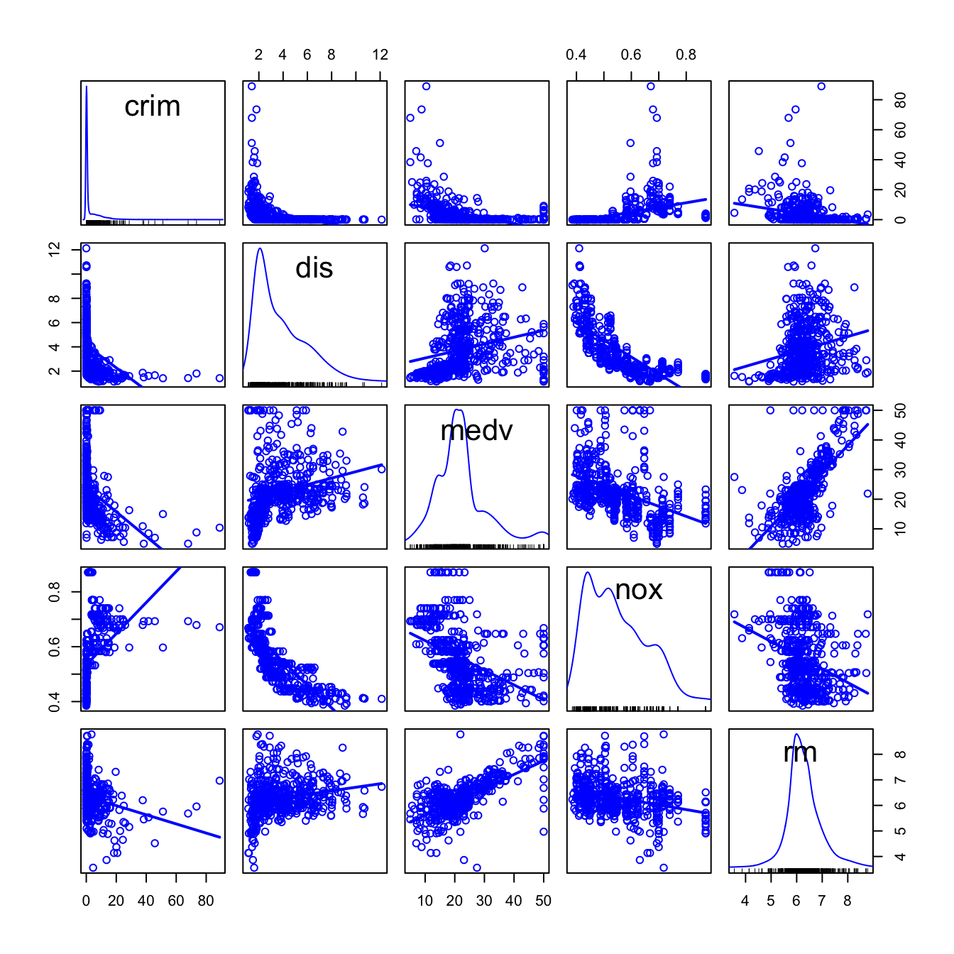
Figure 3.4: Scatterplot matrix for crim, dis, medv, nox and rm from the Boston dataset.
The diagonal panels are showing an estimate of the unknown density of each variable. Note the peculiar distribution of crim, very concentrated at zero, and the asymmetry in medv, with a second mode associated to the most expensive properties. Inspecting the individual panels, it is clear that some nonlinearity exists in the data. For simplicity, we disregard that analysis for the moment (but see the final exercise).
Let’s fit a multiple linear regression for explaining medv. There are a good number of variables now and some of them might be of little use for predicting medv. However, there is no clear intuition of which predictors will yield better explanations of medv with the information at hand. Therefore, we can start by doing a linear model on all the predictors:
modHouse <- lm(medv ~ ., data = Boston)
summary(modHouse)
##
## Call:
## lm(formula = medv ~ ., data = Boston)
##
## Residuals:
##     Min      1Q  Median      3Q     Max
## -15.595  -2.730  -0.518   1.777  26.199
##
## Coefficients:
##               Estimate Std. Error t value Pr(>|t|)
## (Intercept)  3.646e+01  5.103e+00   7.144 3.28e-12 ***
## crim        -1.080e-01  3.286e-02  -3.287 0.001087 **
## zn           4.642e-02  1.373e-02   3.382 0.000778 ***
## indus        2.056e-02  6.150e-02   0.334 0.738288
## chas         2.687e+00  8.616e-01   3.118 0.001925 **
## nox         -1.777e+01  3.820e+00  -4.651 4.25e-06 ***
## rm           3.810e+00  4.179e-01   9.116  < 2e-16 ***
## age          6.922e-04  1.321e-02   0.052 0.958229
## dis         -1.476e+00  1.995e-01  -7.398 6.01e-13 ***
## rad          3.060e-01  6.635e-02   4.613 5.07e-06 ***
## tax         -1.233e-02  3.760e-03  -3.280 0.001112 **
## ptratio     -9.527e-01  1.308e-01  -7.283 1.31e-12 ***
## black        9.312e-03  2.686e-03   3.467 0.000573 ***
## lstat       -5.248e-01  5.072e-02 -10.347  < 2e-16 ***
## ---
## Signif. codes:  0 '***' 0.001 '**' 0.01 '*' 0.05 '.' 0.1 ' ' 1
##
## Residual standard error: 4.745 on 492 degrees of freedom
## Multiple R-squared:  0.7406, Adjusted R-squared:  0.7338
## F-statistic: 108.1 on 13 and 492 DF,  p-value: < 2.2e-16
There are a couple of non-significant variables, but so far the model has an \(R^2=0.74\) and the fitted coefficients are sensible with what it would be expected. For example, crim, tax, ptratio and nox have negative effects on medv, while rm, rad and chas have positive. However, the non-significant coefficients are not improving significantly the model, but only adding artificial noise and decreasing the overall accuracy of the coefficient estimates!
Let’s polish a little bit the previous model. Instead of removing manually each non-significant variable to reduce the complexity, we employ an automatic tool in R called stepwise model selection. It has different flavors, that we will see in detail in Section 3.7, but essentially this powerful tool usually ends up selecting “a” best model: a model that delivers the maximum fit with the minimum number of variables.
The stepwise model selection is located at 'Models' -> 'Stepwise model selection...' and is always applied on the active model. Apply it with the default options to modBest:
modBest <- stepwise(modHouse, direction = 'backward/forward', criterion = 'BIC')
##
## Direction:  backward/forward
## Criterion:  BIC
##
## Start:  AIC=1648.81
## medv ~ crim + zn + indus + chas + nox + rm + age + dis + rad +
##     tax + ptratio + black + lstat
##
##           Df Sum of Sq   RSS    AIC
## - age      1      0.06 11079 1642.6
## - indus    1      2.52 11081 1642.7
## <none>                 11079 1648.8
## - chas     1    218.97 11298 1652.5
## - tax      1    242.26 11321 1653.5
## - crim     1    243.22 11322 1653.6
## - zn       1    257.49 11336 1654.2
## - black    1    270.63 11349 1654.8
## - rad      1    479.15 11558 1664.0
## - nox      1    487.16 11566 1664.4
## - ptratio  1   1194.23 12273 1694.4
## - dis      1   1232.41 12311 1696.0
## - rm       1   1871.32 12950 1721.6
## - lstat    1   2410.84 13490 1742.2
##
## Step:  AIC=1642.59
## medv ~ crim + zn + indus + chas + nox + rm + dis + rad + tax +
##     ptratio + black + lstat
##
##           Df Sum of Sq   RSS    AIC
## - indus    1      2.52 11081 1636.5
## <none>                 11079 1642.6
## - chas     1    219.91 11299 1646.3
## - tax      1    242.24 11321 1647.3
## - crim     1    243.20 11322 1647.3
## - zn       1    260.32 11339 1648.1
## - black    1    272.26 11351 1648.7
## + age      1      0.06 11079 1648.8
## - rad      1    481.09 11560 1657.9
## - nox      1    520.87 11600 1659.6
## - ptratio  1   1200.23 12279 1688.4
## - dis      1   1352.26 12431 1694.6
## - rm       1   1959.55 13038 1718.8
## - lstat    1   2718.88 13798 1747.4
##
## Step:  AIC=1636.48
## medv ~ crim + zn + chas + nox + rm + dis + rad + tax + ptratio +
##     black + lstat
##
##           Df Sum of Sq   RSS    AIC
## <none>                 11081 1636.5
## - chas     1    227.21 11309 1640.5
## - crim     1    245.37 11327 1641.3
## - zn       1    257.82 11339 1641.9
## - black    1    270.82 11352 1642.5
## + indus    1      2.52 11079 1642.6
## - tax      1    273.62 11355 1642.6
## + age      1      0.06 11081 1642.7
## - rad      1    500.92 11582 1652.6
## - nox      1    541.91 11623 1654.4
## - ptratio  1   1206.45 12288 1682.5
## - dis      1   1448.94 12530 1692.4
## - rm       1   1963.66 13045 1712.8
## - lstat    1   2723.48 13805 1741.5
Note the different steps: it starts with the full model and, when + is shown, it means that the variable is excluded at that step. The procedure seeks to minimize an information criterion (BIC or AIC)21. An information criterion balances the fitness of a model with the number of predictors employed. Hence, it determines objectively the best model: the one that minimizes the information criterion. Remember to save the output to a variable if you want to have the final model (you need to do this in R)!
The summary of the final model is:
summary(modBest)
##
## Call:
## lm(formula = medv ~ crim + zn + chas + nox + rm + dis + rad +
##     tax + ptratio + black + lstat, data = Boston)
##
## Residuals:
##      Min       1Q   Median       3Q      Max
## -15.5984  -2.7386  -0.5046   1.7273  26.2373
##
## Coefficients:
##               Estimate Std. Error t value Pr(>|t|)
## (Intercept)  36.341145   5.067492   7.171 2.73e-12 ***
## crim         -0.108413   0.032779  -3.307 0.001010 **
## zn            0.045845   0.013523   3.390 0.000754 ***
## chas          2.718716   0.854240   3.183 0.001551 **
## nox         -17.376023   3.535243  -4.915 1.21e-06 ***
## rm            3.801579   0.406316   9.356  < 2e-16 ***
## dis          -1.492711   0.185731  -8.037 6.84e-15 ***
## rad           0.299608   0.063402   4.726 3.00e-06 ***
## tax          -0.011778   0.003372  -3.493 0.000521 ***
## ptratio      -0.946525   0.129066  -7.334 9.24e-13 ***
## black         0.009291   0.002674   3.475 0.000557 ***
## lstat        -0.522553   0.047424 -11.019  < 2e-16 ***
## ---
## Signif. codes:  0 '***' 0.001 '**' 0.01 '*' 0.05 '.' 0.1 ' ' 1
##
## Residual standard error: 4.736 on 494 degrees of freedom
## Multiple R-squared:  0.7406, Adjusted R-squared:  0.7348
## F-statistic: 128.2 on 11 and 494 DF,  p-value: < 2.2e-16
Let’s compute the confidence intervals at level \(\alpha=0.05\):
confint(modBest)
##                     2.5 %       97.5 %
## (Intercept)  26.384649126  46.29764088
## crim         -0.172817670  -0.04400902
## zn            0.019275889   0.07241397
## chas          1.040324913   4.39710769
## nox         -24.321990312 -10.43005655
## rm            3.003258393   4.59989929
## dis          -1.857631161  -1.12779176
## rad           0.175037411   0.42417950
## tax          -0.018403857  -0.00515209
## ptratio      -1.200109823  -0.69293932
## black         0.004037216   0.01454447
## lstat        -0.615731781  -0.42937513
We have quantified the influence of the predictor variables in the housing prices (Q1) and we can conclude that, in the final model and with confidence level \(\alpha=0.05\):
chas,age,radandblackhave a significantly positive influence onmedv.nox,dis,tax,pratioandlstathave a significantly negative influence onmedv.
The model employed in Harrison and Rubinfeld (1978) is different from modBest. In the paper, several nonlinear transformations of the predictors (remember Section 2.8) and the response are done to improve the linear fit. Also, different units are used for medv, black, lstat and nox. The authors considered these variables:
- Response:
log(1000 * medv) - Linear predictors:
age,black / 1000(this variable corresponds to their \((B-0.63)^2\)),tax,ptratio,crim,zn,indusandchas. - Nonlinear predictors:
rm^2,log(dis),log(rad),log(lstat / 100)and(10 * nox)^2.
Do the following:
Check if the model with such predictors corresponds to the one in the first column, Table VII, page 100 of Harrison and Rubinfeld (1978) (open-access paper available here). To do so, Save this model as
modelHarrisonand summarize it. Hint: the formula should be something likeI(log(1000 * medv)) ~ age + I(black / 1000) + ... + I(log(lstat / 100)) + I((10 * nox)^2).Make a
stepwiseselection of the variables inmodelHarrison(use defaults) and save it asmodelHarrisonSel. Summarize it.Which model has a larger \(R^2\)? And adjusted \(R^2\)? Which is simpler and has more significant coefficients?
References
In Ashenfelter, Ashmore and Lalonde (1995), this variable is expressed relative to the price of the 1961 vintage, regarded as the best one ever recorded. In other words, they consider
Price - 8.4937as the price variable.↩︎If you wanted to do so, you will need the function
I()for indicating that+is not including predictors in the model, but is acting as a sum operator:Price ~ I(Age + AGST + FrancePop + HarvestRain + WinterRain).↩︎The \(R^2\) for the multiple linear regression \(Y=\beta_0+\beta_1X_1+\cdots+\beta_kX_k+\varepsilon\) is not the sum of the \(R^2\)’s for the simple linear regressions \(Y=\beta_0+\beta_jX_j+\varepsilon\), \(j=1,\ldots,k\).↩︎
But be aware of the changes in units for
medv,black,lstatandnox.↩︎Although note that the printed messages always display
'AIC'even if you choose'BIC'.↩︎