6.2 Agglomerative hierarchical clustering
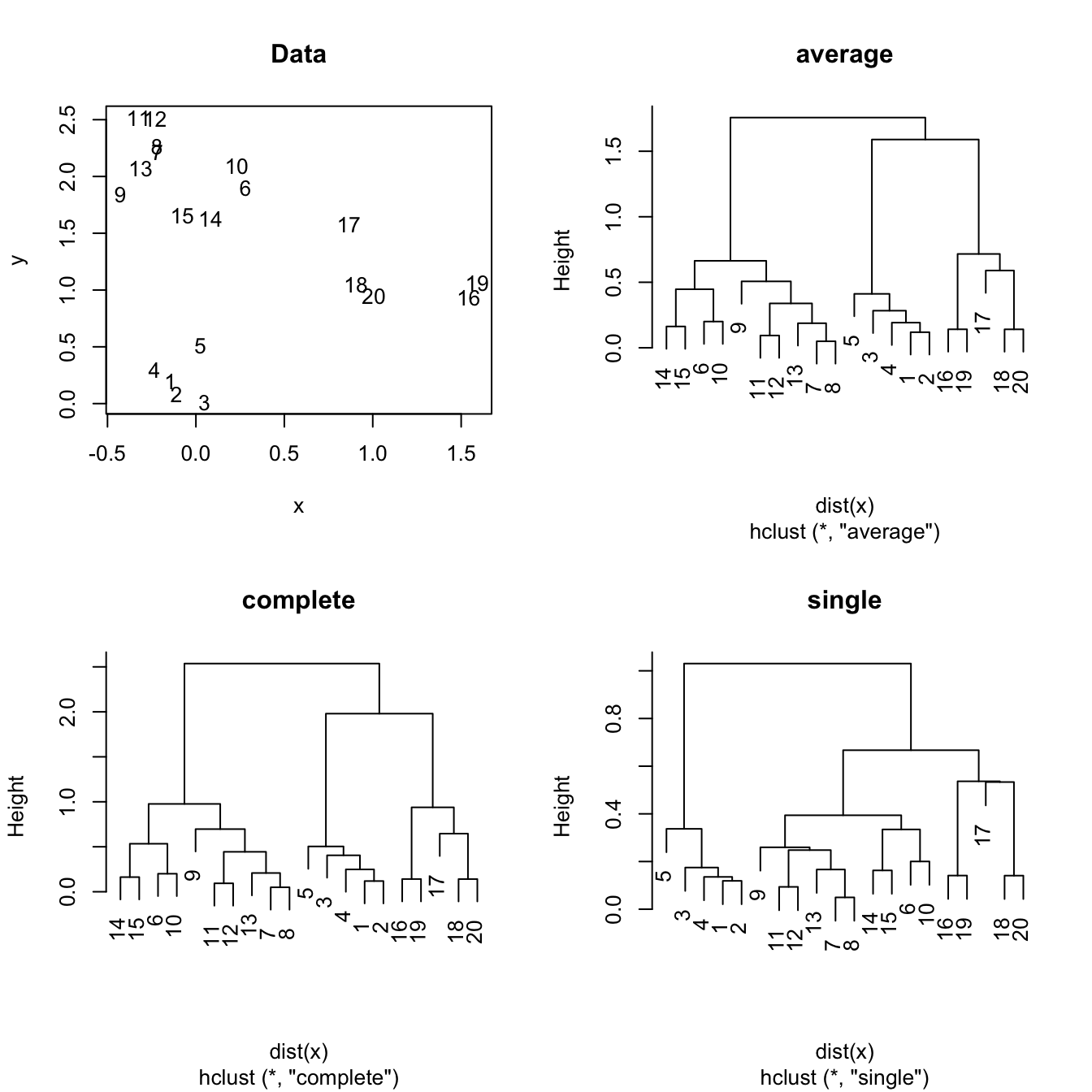
Figure 6.2: The hierarchical clustering for a two-dimensional dataset with complete, single and average linkages.
Hierarchical clustering starts by considering that each observation is its own cluster, and then merges sequentially the clusters with a lower degree of dissimilarity \(d\) (the lower the similarity, the larger the similarity). For example, if there are three clusters, \(A\), \(B\) and \(C\), and their dissimilarities are \(d(A,B)=0.1\), \(d(A,C)=0.5\), \(d(B,C)=0.9\), then the three clusters will be reduced to just two: \((A,B)\) and \(C\).
The advantages of hierarchical clustering are several:
- We do not need to specify a fixed number of clusters \(k\).
- The clusters are naturally nested within each other, something that does not happen in \(k\)-means. Is possible to visualize this nested structure throughout the dendrogram.
- It can deal with categorical variables, throughout the specification of proper dissimilarity measures. In particular, it can deal with numerical variables using the Euclidean distance.
The linkage employed by hierarchical clustering refers to how the cluster are fused:
- Complete. Takes the maximal dissimilarity between all the pairwise dissimilarities between the observations in cluster A and cluster B.
- Single. Takes the minimal dissimilarity between all the pairwise dissimilarities between the observations in cluster A and cluster B.
- Average. Takes the average dissimilarity between all the pairwise dissimilarities between the observations in cluster A and cluster B.
Hierarchical clustering is quite sensible to the kind of dissimilarity employed and the kind of linkage used. In addition, the hierarchical property might force the clusters to unnatural behaviors. Particularly, single linkage may result in extended, chained clusters in which a single observation is added at a new level. As a consequence, complete and average are usually recommended in practice.
Let’s illustrate how to perform hierarchical clustering in laligaStd.
# Compute dissimilarity matrix - in this case Euclidean distance
d <- dist(laligaStd)

# Hierarchical clustering with complete linkage
treeComp <- hclust(d, method = "complete")
plot(treeComp)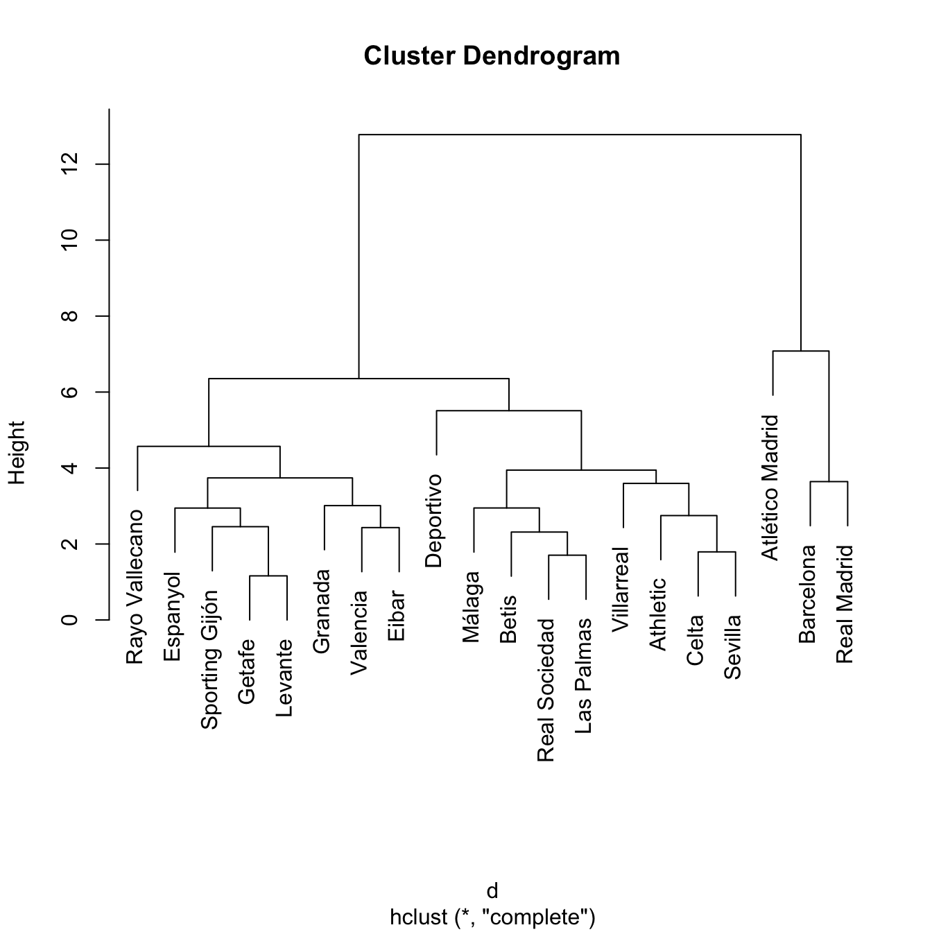
# With average linkage
treeAve <- hclust(d, method = "average")
plot(treeAve)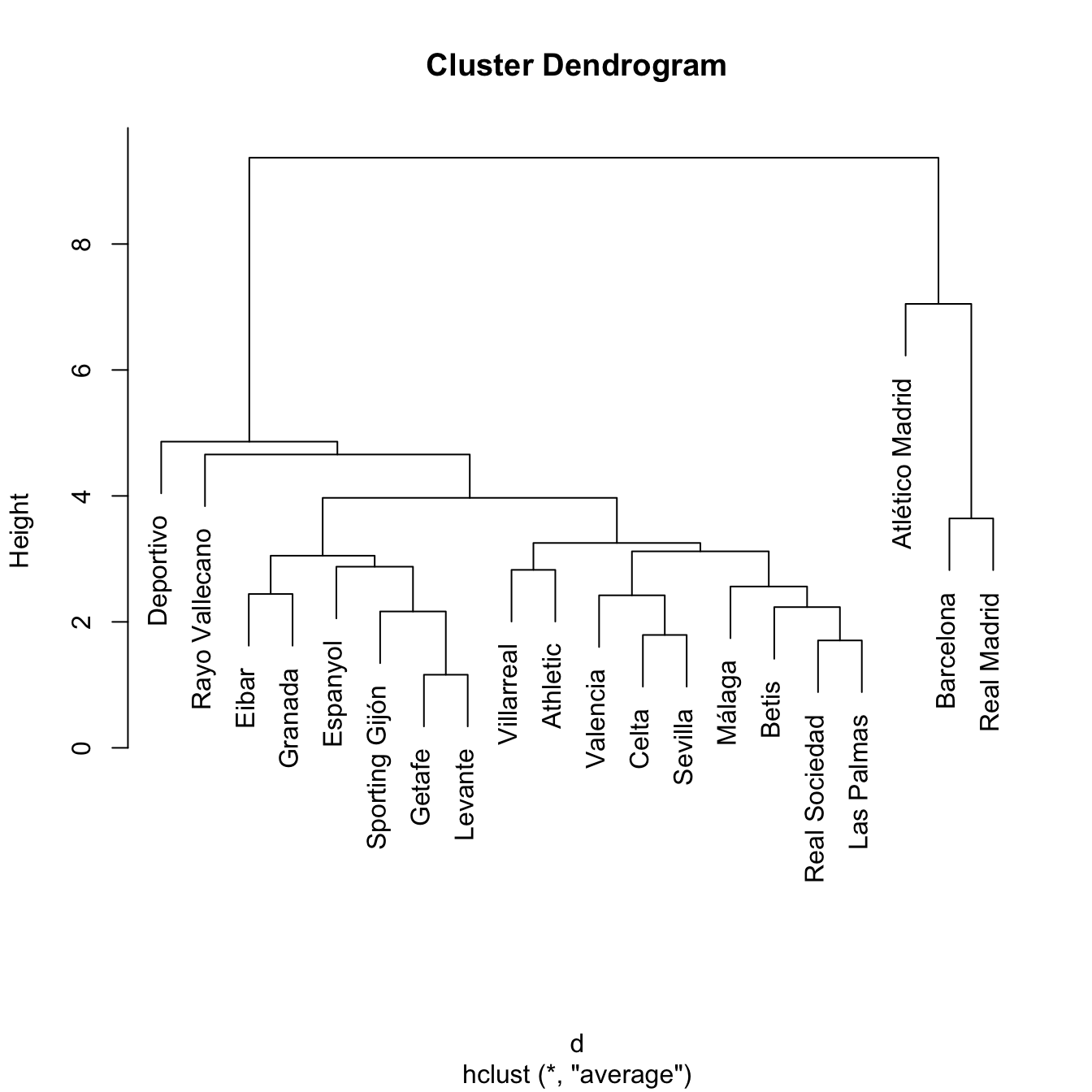
# With single linkage
treeSingle <- hclust(d, method = "single")
plot(treeSingle) # Chaining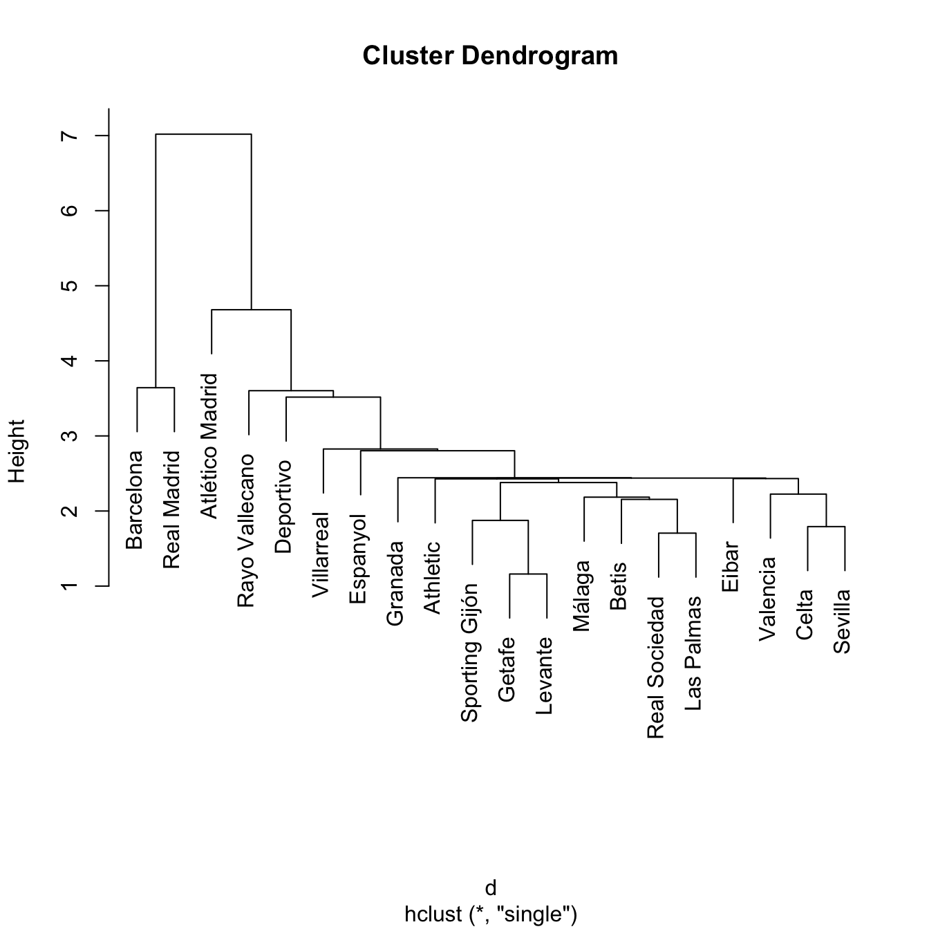
# Set the number of clusters after inspecting visually the dendrogram for "long"
# groups of hanging leaves
# These are the cluster assignments
cutree(treeComp, k = 2) # (Barcelona, Real Madrid) and (rest)
##       Barcelona     Real Madrid Atlético Madrid      Villarreal        Athletic
##               1               1               1               2               2
##           Celta         Sevilla          Málaga   Real Sociedad           Betis
##               2               2               2               2               2
##      Las Palmas        Valencia           Eibar        Espanyol       Deportivo
##               2               2               2               2               2
##         Granada  Sporting Gijón  Rayo Vallecano          Getafe         Levante
##               2               2               2               2               2
cutree(treeComp, k = 3) # (Barcelona, Real Madrid), (Atlético Madrid) and (rest)
##       Barcelona     Real Madrid Atlético Madrid      Villarreal        Athletic
##               1               1               2               3               3
##           Celta         Sevilla          Málaga   Real Sociedad           Betis
##               3               3               3               3               3
##      Las Palmas        Valencia           Eibar        Espanyol       Deportivo
##               3               3               3               3               3
##         Granada  Sporting Gijón  Rayo Vallecano          Getafe         Levante
##               3               3               3               3               3

# Compare differences - treeComp makes more sense than treeAve
cutree(treeComp, k = 4)
##       Barcelona     Real Madrid Atlético Madrid      Villarreal        Athletic
##               1               1               2               3               3
##           Celta         Sevilla          Málaga   Real Sociedad           Betis
##               3               3               3               3               3
##      Las Palmas        Valencia           Eibar        Espanyol       Deportivo
##               3               4               4               4               3
##         Granada  Sporting Gijón  Rayo Vallecano          Getafe         Levante
##               4               4               4               4               4
cutree(treeAve, k = 4)
##       Barcelona     Real Madrid Atlético Madrid      Villarreal        Athletic
##               1               1               2               3               3
##           Celta         Sevilla          Málaga   Real Sociedad           Betis
##               3               3               3               3               3
##      Las Palmas        Valencia           Eibar        Espanyol       Deportivo
##               3               3               3               3               4
##         Granada  Sporting Gijón  Rayo Vallecano          Getafe         Levante
##               3               3               3               3               3

# We can plot the results in the first two PCs, as we did in k-means
cluster <- cutree(treeComp, k = 2)
plot(pca$scores[, 1:2], col = cluster)
text(x = pca$scores[, 1:2], labels = rownames(pca$scores), pos = 3, col = cluster)
cluster <- cutree(treeComp, k = 3)
plot(pca$scores[, 1:2], col = cluster)
text(x = pca$scores[, 1:2], labels = rownames(pca$scores), pos = 3, col = cluster)
cluster <- cutree(treeComp, k = 4)
plot(pca$scores[, 1:2], col = cluster)
text(x = pca$scores[, 1:2], labels = rownames(pca$scores), pos = 3, col = cluster)
If categorical variables are present, replace
 dist by daisy from the cluster package (you need to do first library(cluster)). For example, let’s cluster the iris dataset.
# Load data
data(iris)

# The fifth variable is a factor
head(iris)
##   Sepal.Length Sepal.Width Petal.Length Petal.Width Species
## 1          5.1         3.5          1.4         0.2  setosa
## 2          4.9         3.0          1.4         0.2  setosa
## 3          4.7         3.2          1.3         0.2  setosa
## 4          4.6         3.1          1.5         0.2  setosa
## 5          5.0         3.6          1.4         0.2  setosa
## 6          5.4         3.9          1.7         0.4  setosa

# Compute dissimilarity matrix using the Gower dissimilarity measure
# This dissimilarity is able to handle both numerical and categorical variables
# daisy automatically detects whether there are factors present in the data and
# applies Gower (otherwise it applies the Euclidean distance)
library(cluster)
d <- daisy(iris)
tree <- hclust(d)

# 3 main clusters
plot(tree)
# The clusters correspond to the Species
cutree(tree, k = 3)
##   [1] 1 1 1 1 1 1 1 1 1 1 1 1 1 1 1 1 1 1 1 1 1 1 1 1 1 1 1 1 1 1 1 1 1 1 1 1 1
##  [38] 1 1 1 1 1 1 1 1 1 1 1 1 1 2 2 2 2 2 2 2 2 2 2 2 2 2 2 2 2 2 2 2 2 2 2 2 2
##  [75] 2 2 2 2 2 2 2 2 2 2 2 2 2 2 2 2 2 2 2 2 2 2 2 2 2 2 3 3 3 3 3 3 3 3 3 3 3
## [112] 3 3 3 3 3 3 3 3 3 3 3 3 3 3 3 3 3 3 3 3 3 3 3 3 3 3 3 3 3 3 3 3 3 3 3 3 3
## [149] 3 3
table(iris$Species, cutree(tree, k = 3))
##
##               1  2  3
##   setosa     50  0  0
##   versicolor  0 50  0
##   virginica   0  0 50
Performing hierarchical clustering in practice depends on several decisions that may have big consequences on the final output:
- What kind of dissimilarity and linkage should be employed? Not a single answer: try several and compare.
- Where to cut the dendrogram? The general advice is to look for groups of branches hanging for a long space and cut on their top.
Despite the general advice, there is not a single and best solution for the previous questions. What is advisable in practice is to analyze several choices, report the general patterns that arise and the different features of the data the methods expose.
Hierarchical clustering can also be performed through the help of R Commander. To do so, go to 'Statistics' -> 'Dimensional Analysis' -> 'Clustering' -> 'Hierar...'. If you do this for the USArrests dataset after rescaling, you should get something like this:
HClust.1 <- hclust(dist(model.matrix(~-1 + Assault + Murder + Rape + UrbanPop,
                                     USArrests)), method = "complete")
plot(HClust.1, main = "Cluster Dendrogram for Solution HClust.1",
     xlab = "Observation Number in Data Set USArrests",
     sub = "Method=complete; Distance=euclidian")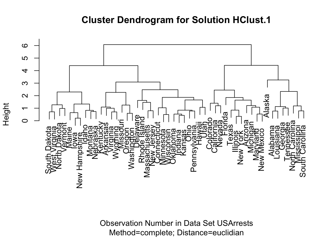
Import the eurojob (download) dataset and standardize it properly. Perform a hierarchical clustering analysis for the three kind of linkages seen.