3.3 Assumptions of the model
Some probabilistic assumptions are required for performing inference on the model parameters. In other words, to infer properties about the unknown population coefficients \(\boldsymbol{\beta}\) from the sample \((\mathbf{X}_1, Y_1),\ldots,(\mathbf{X}_n, Y_n)\).
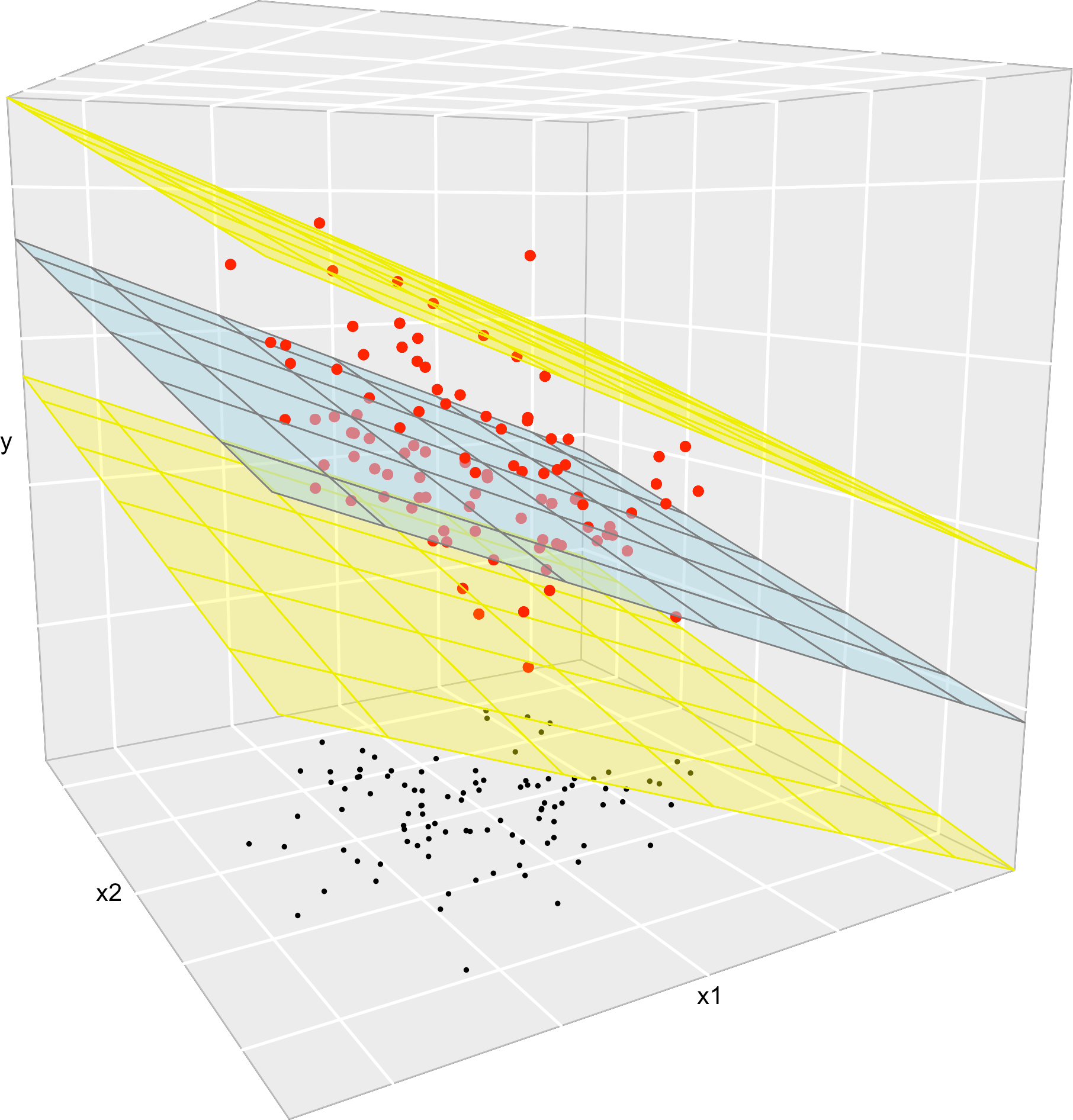
Figure 3.7: The key concepts of the multiple linear model when \(k=2\). The space between the yellow planes denotes where the \(95\%\) of the data is, according to the model.
The assumptions of the multiple linear model are an extension of the simple linear model:
- Linearity: \(\mathbb{E}[Y|X_1=x_1,\ldots,X_k=x_k]=\beta_0+\beta_1x_1+\cdots+\beta_kx_k\).
- Homoscedasticity: \(\mathbb{V}\text{ar}(\varepsilon_i)=\sigma^2\), with \(\sigma^2\) constant for \(i=1,\ldots,n\).
- Normality: \(\varepsilon_i\sim\mathcal{N}(0,\sigma^2)\) for \(i=1,\ldots,n\).
- Independence of the errors: \(\varepsilon_1,\ldots,\varepsilon_n\) are independent (or uncorrelated, \(\mathbb{E}[\varepsilon_i\varepsilon_j]=0\), \(i\neq j\), since they are assumed to be normal).
A good one-line summary of the linear model is the following (independence is assumed) \[\begin{align} Y|(X_1=x_1,\ldots,X_k=x_k)\sim \mathcal{N}(\beta_0+\beta_1x_1+\cdots+\beta_kx_k,\sigma^2).\tag{3.5} \end{align}\]
Recall:
Compared with simple liner regression, the only different assumption is linearity.
Nothing is said about the distribution of \(X_1,\ldots,X_k\). They could be deterministic or random. They could be discrete or continuous.
\(X_1,\ldots,X_k\) are not required to be independent between them.
\(Y\) has to be continuous, since the errors are normal – recall (2.1).
Figure 3.8 represents situations where the assumptions of the model are respected and violated, for the situation with two predictors. Clearly, the inspection of the scatterplots for identifying strange patterns is more complicated than in simple linear regression – and here we are dealing only with two predictors. In Section 3.8 we will see more sophisticated methods for checking whether the assumptions hold or not for an arbitrary number of predictors.
Figure 3.8: Valid (all the assumptions are verified) and problematic (a single assumption does not hold) multiple linear models, when there are two predictors. Application also available here.
To conclude this section, let’s see how to make a 3D scatterplot with the regression plane, in order to evaluate visually how good the fit of the model is. We will do it with the iris dataset, that can be imported in R simply by running data(iris). In R Commander go to 'Graphs' -> '3D Graphs' -> '3D scatterplot...'. A window like Figures 3.9 and 3.10 will pop-up. The options are similar to the ones for 'Graphs' -> 'Scatterplot...'.
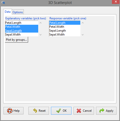
Figure 3.9: 3D scatterplot window, 'Data' panel.
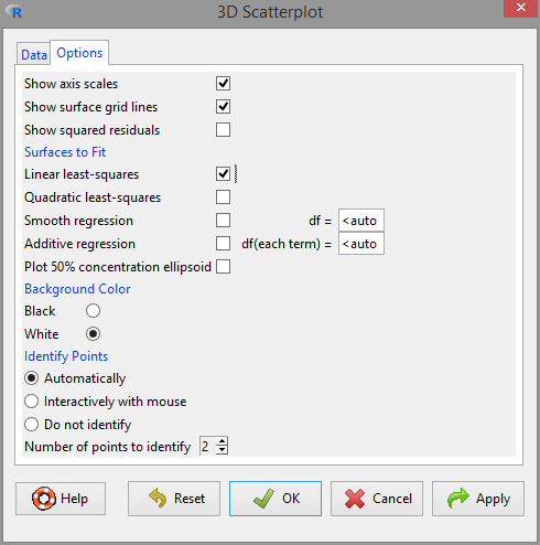
Figure 3.10: 3D scatterplot window, 'Options' panel. Remember to tick the 'Linear least-squares fit' box in order to display the fitted regression plane.
If you select the options as shown in Figures 3.9 and 3.10, you should get something like this:
data(iris)
scatter3d(Petal.Length ~ Petal.Width + Sepal.Length, data = iris, fit = "linear",
          residuals = TRUE, bg = "white", axis.scales = TRUE, grid = TRUE,
          ellipsoid = FALSE, id.method = 'mahal', id.n = 2)
## Loading required namespace: mgcv