6.1 \(k\)-means clustering
The \(k\)-means clustering looks for \(k\) clusters in the data such that they are as compact as possible and as separated as possible. In clustering terminology, the clusters minimize the with-in cluster variation with respect to the cluster centroid while they maximize the between cluster variation among clusters. The distance used for measuring proximity is the usual Euclidean distance between points. As a consequence, this clustering method tend to yield spherical or rounded clusters and is not adequate for categorical variables.
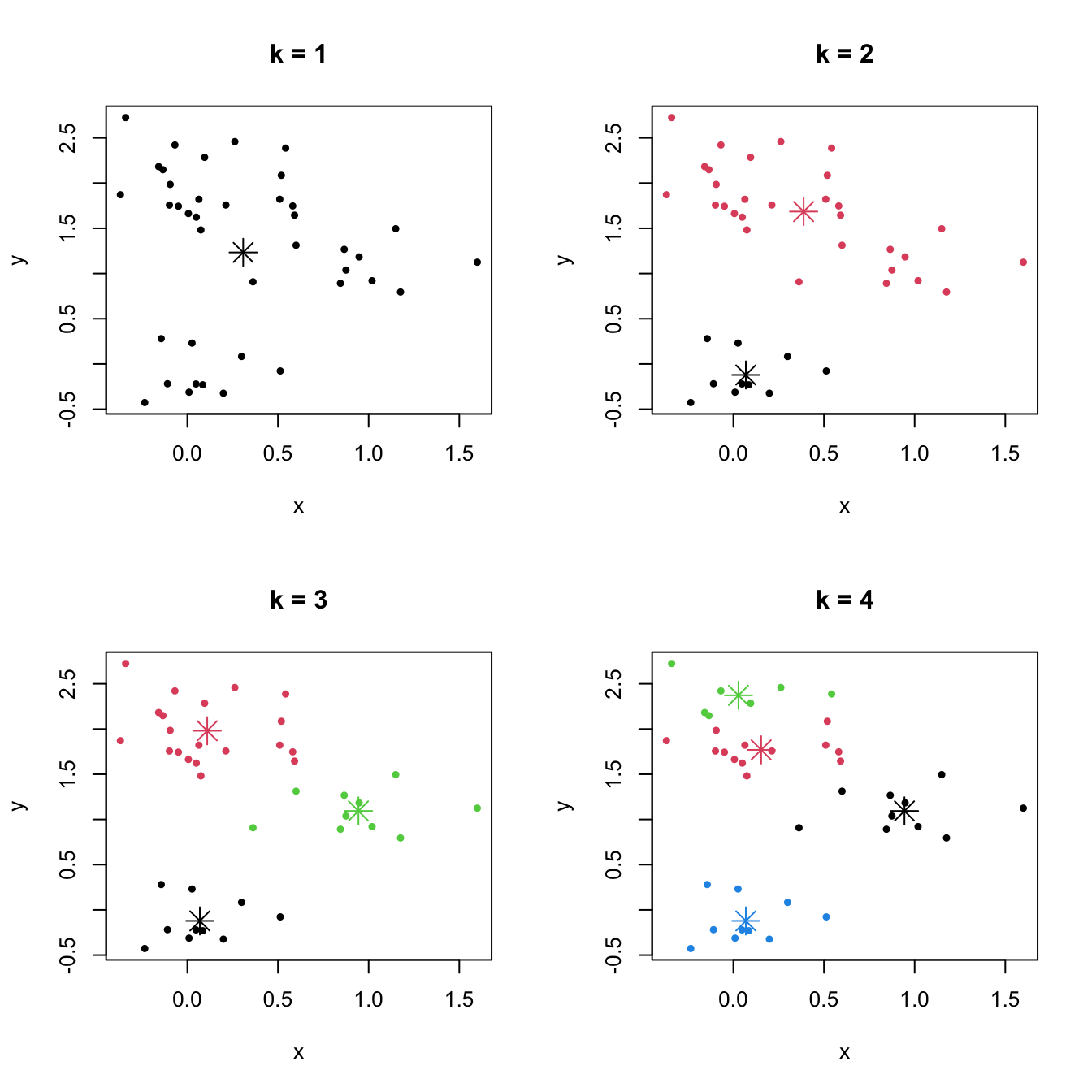
Figure 6.1: The \(k\)-means partitions for a two-dimensional dataset with \(k=1,2,3,4\). Centers of each cluster are displayed with an asterisk.
Let’s analyze the possible clusters in a smaller subset of La Liga 2015/2016 (download) dataset, where the results can be easily visualized. To that end, import the data as laliga.
# We consider only a smaller dataset (Points and Yellow.cards)
head(laliga, 2)
##             Points Matches Wins Draws Loses Goals.scored Goals.conceded
## Barcelona       91      38   29     4     5          112             29
## Real Madrid     90      38   28     6     4          110             34
##             Difference.goals Percentage.scored.goals Percentage.conceded.goals
## Barcelona                 83                    2.95                      0.76
## Real Madrid               76                    2.89                      0.89
##             Shots Shots.on.goal Penalties.scored Assistances Fouls.made
## Barcelona     600           277               11          79        385
## Real Madrid   712           299                6          90        420
##             Matches.without.conceding Yellow.cards Red.cards Offsides
## Barcelona                          18           66         1      120
## Real Madrid                        14           72         5      114
pointsCards <-  laliga[, c(1, 17)]
plot(pointsCards)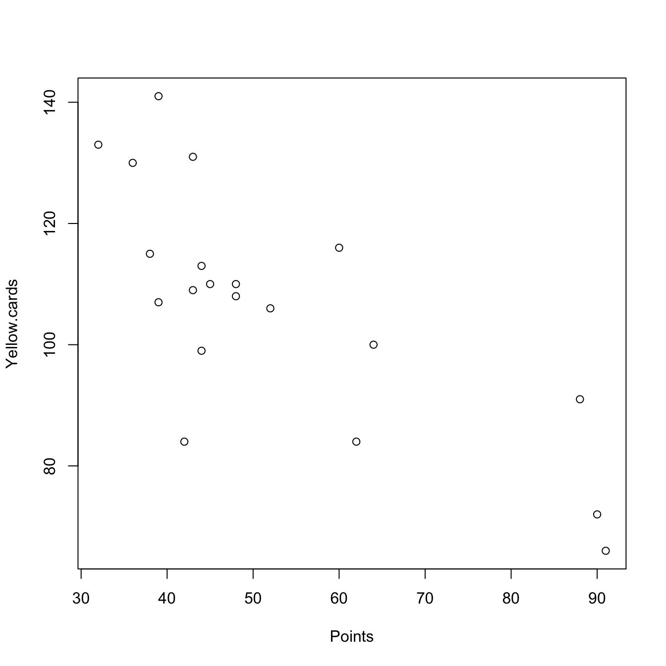
# kmeans uses a random initialization of the clusters, so the results may vary
# from one call to another. We use set.seed() to have reproducible outputs.
set.seed(2345678)

# kmeans call:
# - centers is the k, the number of clusters.
# - nstart indicates how many different starting assignments should be considered
# (useful for avoiding suboptimal clusterings)
k <- 2
km <- kmeans(pointsCards, centers = k, nstart = 20)

# What is inside km?
km
## K-means clustering with 2 clusters of sizes 4, 16
##
## Cluster means:
##    Points Yellow.cards
## 1 82.7500        78.25
## 2 44.8125       113.25
##
## Clustering vector:
##       Barcelona     Real Madrid Atlético Madrid      Villarreal        Athletic
##               1               1               1               2               1
##           Celta         Sevilla          Málaga   Real Sociedad           Betis
##               2               2               2               2               2
##      Las Palmas        Valencia           Eibar        Espanyol       Deportivo
##               2               2               2               2               2
##         Granada  Sporting Gijón  Rayo Vallecano          Getafe         Levante
##               2               2               2               2               2
##
## Within cluster sum of squares by cluster:
## [1]  963.500 4201.438
##  (between_SS / total_SS =  62.3 %)
##
## Available components:
##
## [1] "cluster"      "centers"      "totss"        "withinss"     "tot.withinss"
## [6] "betweenss"    "size"         "iter"         "ifault"
str(km)
## List of 9
##  $ cluster     : Named int [1:20] 1 1 1 2 1 2 2 2 2 2 ...
##   ..- attr(*, "names")= chr [1:20] "Barcelona" "Real Madrid" "Atlético Madrid" "Villarreal" ...
##  $ centers     : num [1:2, 1:2] 82.8 44.8 78.2 113.2
##   ..- attr(*, "dimnames")=List of 2
##   .. ..$ : chr [1:2] "1" "2"
##   .. ..$ : chr [1:2] "Points" "Yellow.cards"
##  $ totss       : num 13691
##  $ withinss    : num [1:2] 964 4201
##  $ tot.withinss: num 5165
##  $ betweenss   : num 8526
##  $ size        : int [1:2] 4 16
##  $ iter        : int 1
##  $ ifault      : int 0
##  - attr(*, "class")= chr "kmeans"

# between_SS / total_SS gives a criterion to select k similar to PCA.
# Recall that between_SS / total_SS = 100% if k = n

# Centroids of each cluster
km$centers
##    Points Yellow.cards
## 1 82.7500        78.25
## 2 44.8125       113.25

# Assignments of observations to the k clusters
km$cluster
##       Barcelona     Real Madrid Atlético Madrid      Villarreal        Athletic
##               1               1               1               2               1
##           Celta         Sevilla          Málaga   Real Sociedad           Betis
##               2               2               2               2               2
##      Las Palmas        Valencia           Eibar        Espanyol       Deportivo
##               2               2               2               2               2
##         Granada  Sporting Gijón  Rayo Vallecano          Getafe         Levante
##               2               2               2               2               2

# Plot data with colors according to clusters
plot(pointsCards, col = km$cluster)

# Add the names of the observations above the points
text(x = pointsCards, labels = rownames(pointsCards), col = km$cluster,
     pos = 3, cex = 0.75)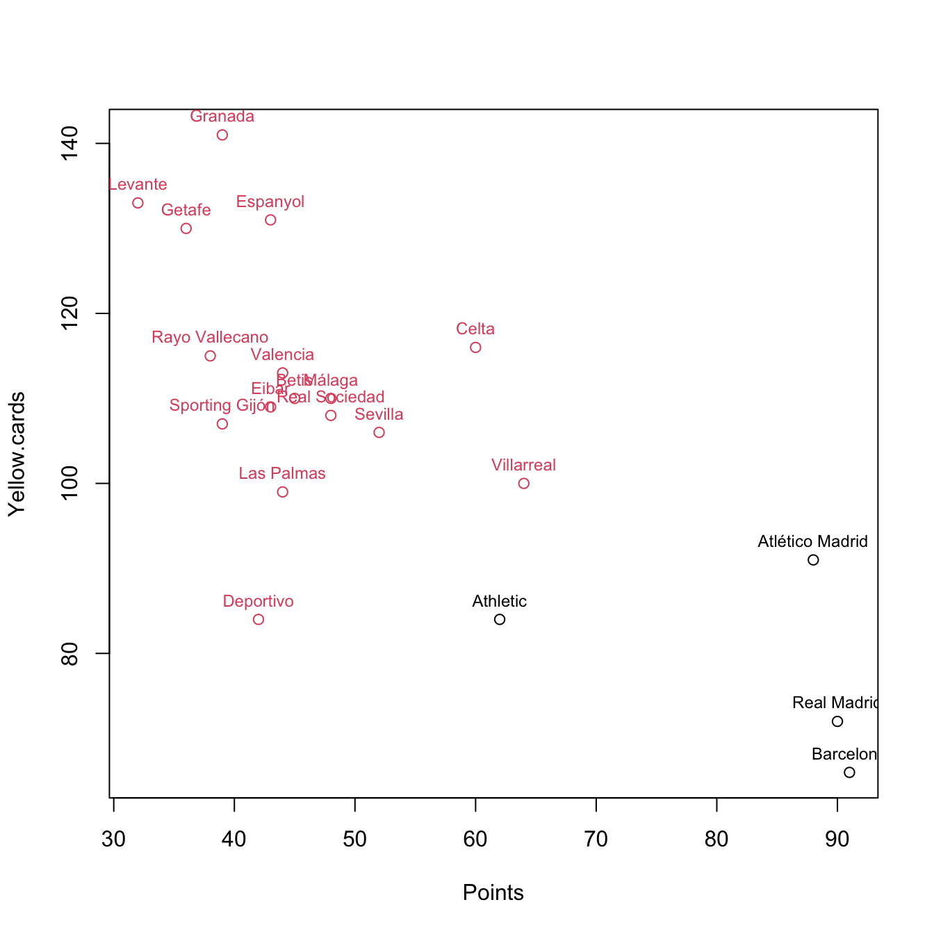
# Clustering with k = 3
k <- 3
set.seed(2345678)
km <- kmeans(pointsCards, centers = k, nstart = 20)
plot(pointsCards, col = km$cluster)
text(x = pointsCards, labels = rownames(pointsCards), col = km$cluster,
     pos = 3, cex = 0.75)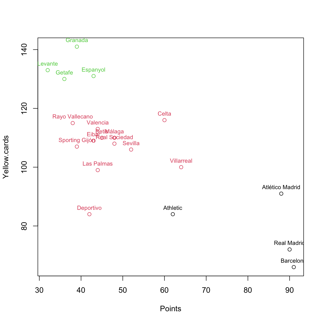
# Clustering with k = 4
k <- 4
set.seed(2345678)
km <- kmeans(pointsCards, centers = k, nstart = 20)
plot(pointsCards, col = km$cluster)
text(x = pointsCards, labels = rownames(pointsCards), col = km$cluster,
     pos = 3, cex = 0.75)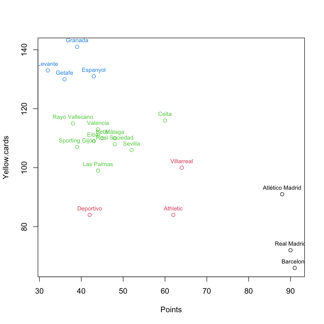
So far, we have only taken the information of two variables for performing clustering. Using PCA, we can visualize the clustering performed with all the available variables in the dataset.
By default, kmeans does not standardize variables, which will affect the clustering result. As a consequence, the clustering of a dataset will be different if one variable is expressed in millions or in tenths. If you want to avoid this distortion, you can use scale to automatically center and standardize a data frame (the result will be a matrix, so you need to transform it to a data frame again).
# Work with standardized data (and remove Matches)
laligaStd <- data.frame(scale(laliga[, -2]))

# Clustering with all the variables - unstandardized data
set.seed(345678)
kme <- kmeans(laliga, centers = 3, nstart = 20)
kme$cluster
##       Barcelona     Real Madrid Atlético Madrid      Villarreal        Athletic
##               1               1               3               2               3
##           Celta         Sevilla          Málaga   Real Sociedad           Betis
##               2               2               2               3               3
##      Las Palmas        Valencia           Eibar        Espanyol       Deportivo
##               3               2               2               2               3
##         Granada  Sporting Gijón  Rayo Vallecano          Getafe         Levante
##               2               2               2               2               2
table(kme$cluster)
##
##  1  2  3
##  2 12  6

# Clustering with all the variables - standardized data
set.seed(345678)
kme <- kmeans(laligaStd, centers = 3, nstart = 20)
kme$cluster
##       Barcelona     Real Madrid Atlético Madrid      Villarreal        Athletic
##               2               2               2               1               1
##           Celta         Sevilla          Málaga   Real Sociedad           Betis
##               1               1               1               1               1
##      Las Palmas        Valencia           Eibar        Espanyol       Deportivo
##               1               1               3               3               1
##         Granada  Sporting Gijón  Rayo Vallecano          Getafe         Levante
##               3               3               3               3               3
table(kme$cluster)
##
##  1  2  3
## 10  3  7

# PCA
pca <- princomp(laliga[, -2], cor = TRUE)
summary(pca)
## Importance of components:
##                           Comp.1    Comp.2     Comp.3     Comp.4     Comp.5
## Standard deviation     3.4372781 1.5514051 1.14023547 0.91474383 0.85799980
## Proportion of Variance 0.6563823 0.1337143 0.07222983 0.04648646 0.04089798
## Cumulative Proportion  0.6563823 0.7900966 0.86232642 0.90881288 0.94971086
##                            Comp.6    Comp.7      Comp.8      Comp.9    Comp.10
## Standard deviation     0.60295746 0.4578613 0.373829925 0.327242606 0.22735805
## Proportion of Variance 0.02019765 0.0116465 0.007763823 0.005949318 0.00287176
## Cumulative Proportion  0.96990851 0.9815550 0.989318830 0.995268148 0.99813991
##                             Comp.11      Comp.12      Comp.13      Comp.14
## Standard deviation     0.1289704085 0.0991188181 0.0837498223 2.860411e-03
## Proportion of Variance 0.0009240759 0.0005458078 0.0003896685 4.545528e-07
## Cumulative Proportion  0.9990639840 0.9996097918 0.9999994603 9.999999e-01
##                             Comp.15      Comp.16      Comp.17 Comp.18
## Standard deviation     1.238298e-03 1.583337e-08 1.154388e-08       0
## Proportion of Variance 8.518782e-08 1.392753e-17 7.403399e-18       0
## Cumulative Proportion  1.000000e+00 1.000000e+00 1.000000e+00       1

# Biplot (the scores of the first two PCs)
biplot(pca)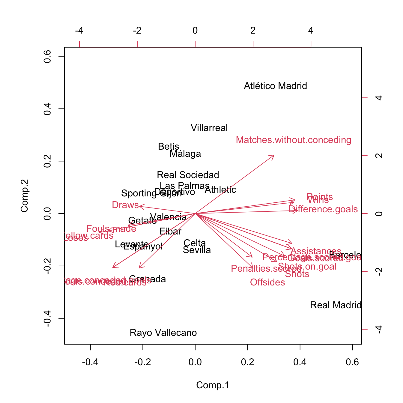
# Redo the biplot with colors indicating the cluster assignments
plot(pca$scores[, 1:2], col = kme$cluster)
text(x = pca$scores[, 1:2], labels = rownames(pca$scores), pos = 3, col = kme$cluster)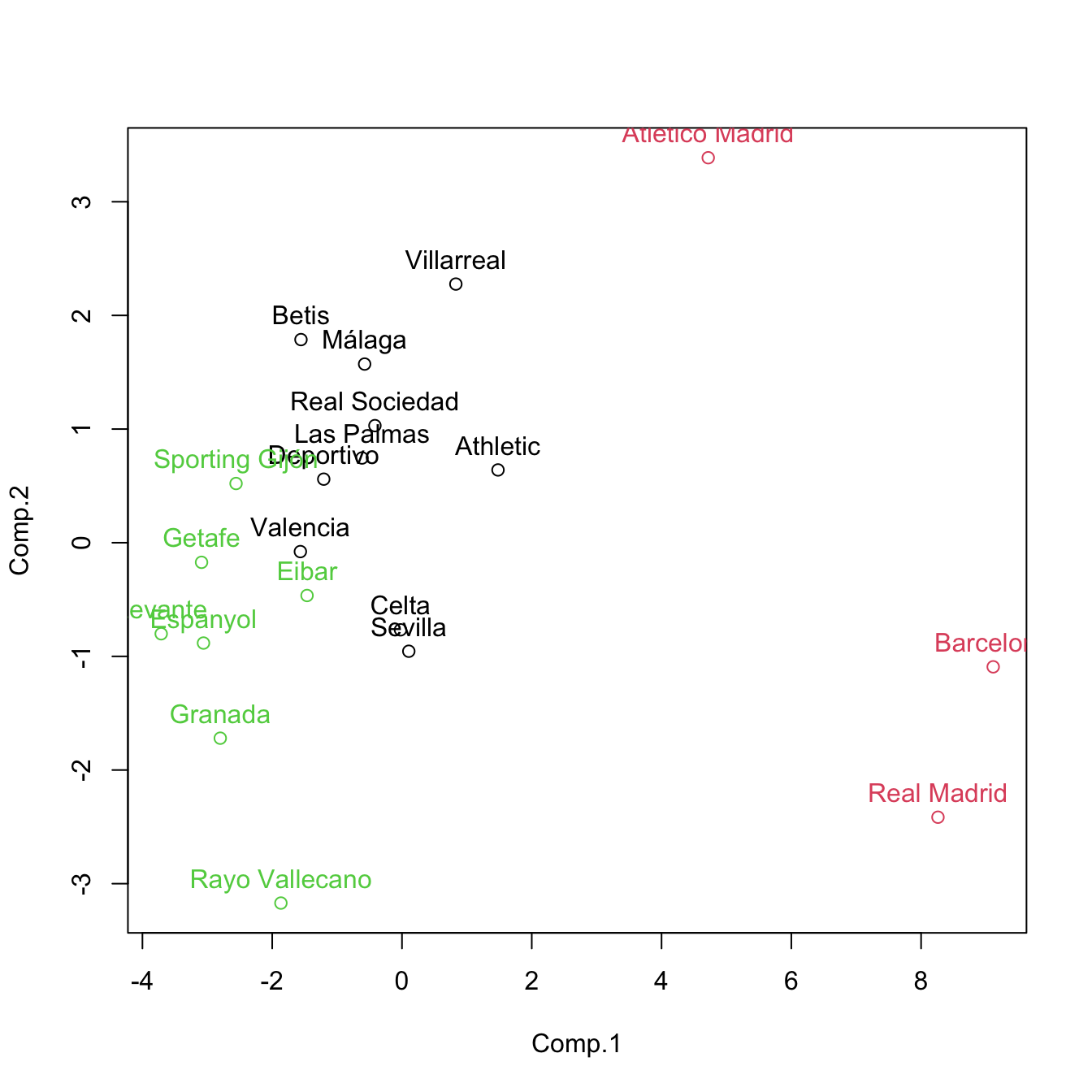
# Recall: this is a visualization with PC1 and PC2 of the clustering done with
# all the variables, not just PC1 and PC2

# Clustering with only the first two PCs - different and less accurate result,
# but still insightful
set.seed(345678)
kme2 <- kmeans(pca$scores[, 1:2], centers = 3, nstart = 20)
plot(pca$scores[, 1:2], col = kme2$cluster)
text(x = pca$scores[, 1:2], labels = rownames(pca$scores), pos = 3, col = kme2$cluster)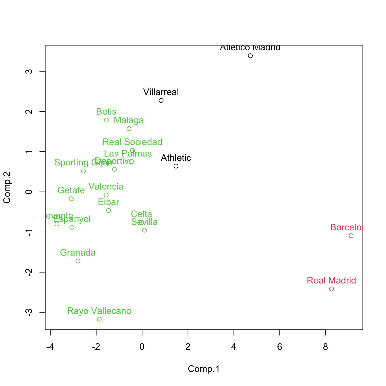
\(k\)-means can also be performed through the help of R Commander. To do so, go to 'Statistics' -> 'Dimensional Analysis' -> 'Clustering' -> 'k-means cluster analysis...'. If you do this for the USArrests dataset after rescaling it, select to 'Assign clusters to the data set' and name the 'Assignment variable' as 'KMeans', you should get something like this:
# Load data and scale it
data(USArrests)
USArrests <- as.data.frame(scale(USArrests))

# Statistics -> Dimensional Analysis -> Clustering -> k-means cluster analysis...
.cluster <-  KMeans(model.matrix(~-1 + Assault + Murder + Rape + UrbanPop, USArrests),
  centers = 2, iter.max = 10, num.seeds = 10)
.cluster$size # Cluster Sizes
## [1] 20 30
.cluster$centers # Cluster Centroids
##   new.x.Assault new.x.Murder new.x.Rape new.x.UrbanPop
## 1     1.0138274     1.004934  0.8469650      0.1975853
## 2    -0.6758849    -0.669956 -0.5646433     -0.1317235
.cluster$withinss # Within Cluster Sum of Squares
## [1] 46.74796 56.11445
.cluster$tot.withinss # Total Within Sum of Squares
## [1] 102.8624
.cluster$betweenss # Between Cluster Sum of Squares
## [1] 93.1376
remove(.cluster)
.cluster <-  KMeans(model.matrix(~-1 + Assault + Murder + Rape + UrbanPop, USArrests),
  centers = 2, iter.max = 10, num.seeds = 10)
.cluster$size # Cluster Sizes
## [1] 20 30
.cluster$centers # Cluster Centroids
##   new.x.Assault new.x.Murder new.x.Rape new.x.UrbanPop
## 1     1.0138274     1.004934  0.8469650      0.1975853
## 2    -0.6758849    -0.669956 -0.5646433     -0.1317235
.cluster$withinss # Within Cluster Sum of Squares
## [1] 46.74796 56.11445
.cluster$tot.withinss # Total Within Sum of Squares
## [1] 102.8624
.cluster$betweenss # Between Cluster Sum of Squares
## [1] 93.1376
biplot(princomp(model.matrix(~-1 + Assault + Murder + Rape + UrbanPop, USArrests)),
  xlabs = as.character(.cluster$cluster))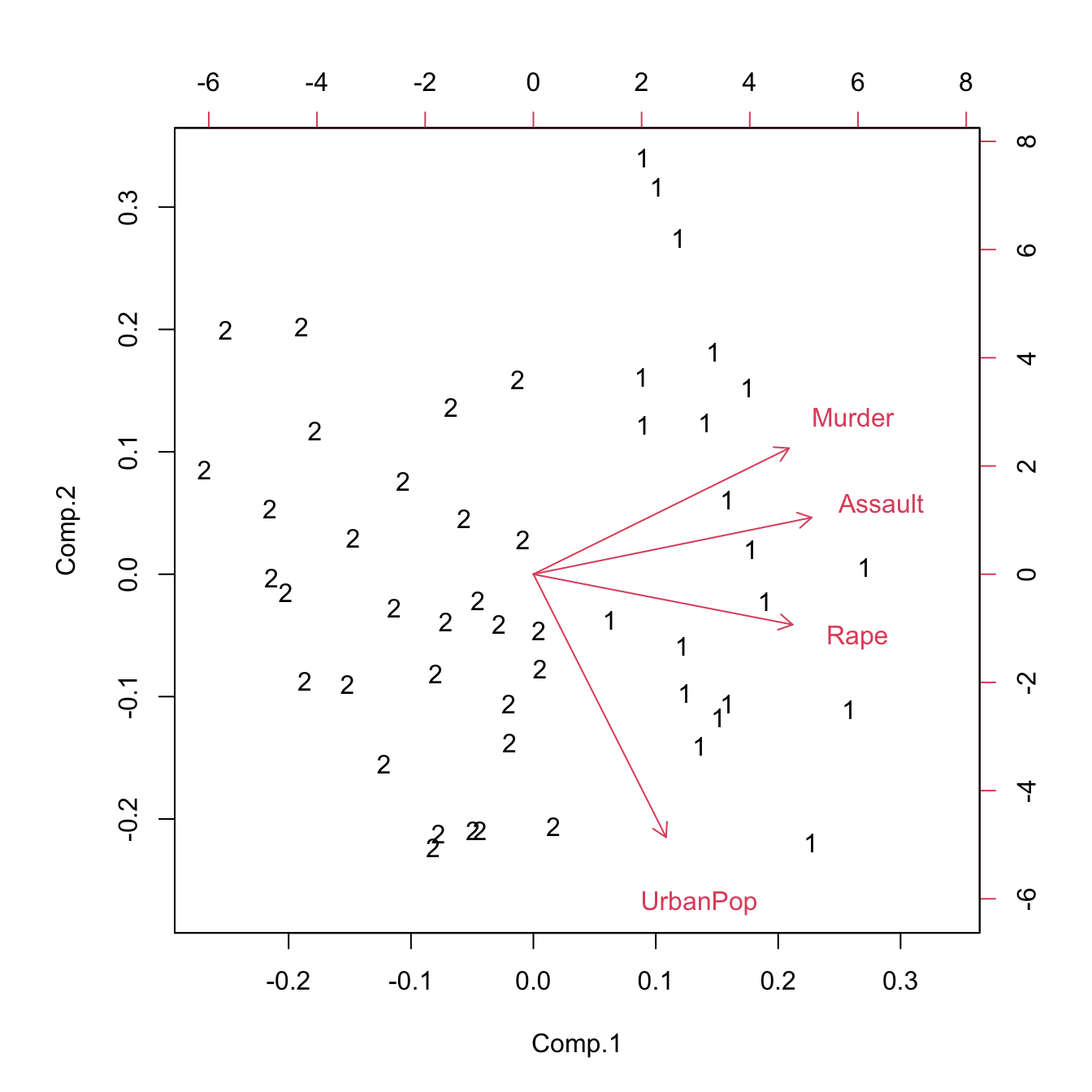
USArrests$KMeans <- assignCluster(model.matrix(~-1 + Assault + Murder + Rape + UrbanPop,
  USArrests), USArrests, .cluster$cluster)
remove(.cluster)
How many clusters \(k\) do we need in practice? There is not a single answer: the advice is to try several and compare. Inspecting the ‘between_SS / total_SS’ for a good trade-off between the number of clusters and the percentage of total variation explained usually gives a good starting point for deciding on \(k\).
For the iris dataset, do sequentially:
- Apply
scaleto the dataset and save it asirisStd. Note: the fifth variable is a factor, so you must skip it. - Fix the seed to 625365712.
- Run \(k\)-means with 20 runs for \(k=2,3,4\). Save the results as
km2,km3andkm4. - Compute the PCA of
irisStd. - Plot the first two scores, colored by the assignments of
km2. - Do the same for
km3andkm4. - Which \(k\) do you think it gives the most sensible partition based on the previous plots?