4.3 Model formulation and estimation by maximum likelihood

As we saw in Section 3.2, the multiple linear model described the relation between the random variables $X_1,\ldots,X_k$ and $Y$ by assuming the linear relation $$\begin{align*} Y = \beta_0 + \beta_1 X_1 + \cdots + \beta_k X_k + \varepsilon. \end{align*}$$ Since we assume $\mathbb{E}[\varepsilon|X_1=x_1,\ldots,X_k=x_k]=0$, the previous equation was equivalent to $$\begin{align} \mathbb{E}[Y|X_1=x_1,\ldots,X_k=x_k]=\beta_0+\beta_1x_1+\cdots+\beta_kx_k,\tag{4.2} \end{align}$$ where $\mathbb{E}[Y|X_1=x_1,\ldots,X_k=x_k]$ is the mean of $Y$ for a particular value of the set of predictors. As remarked in Section 3.3, it was a necessary condition that $Y$ was continuous in order to satisfy the normality of the errors, hence the linear model assumptions. Or in other words, the linear model is designed for a continuous response.

The situation when $Y$ is discrete (naturally ordered values; e.g. number of fails, number of students) or categorical (non-ordered categories; e.g. territorial divisions, ethnic groups) requires a special treatment. The simplest situation is when $Y$ is binary (or dichotomic): it can only take two values, codified for convenience as $1$ (success) and $0$ (failure). For example, in the Challenger case study we used fail.field as an indicator of whether “there was at least an incident with the O-rings” (1 = yes, 0 = no). For binary variables there is no fundamental distinction between the treatment of discrete and categorical variables.

More formally, a binary variable is known as a Bernoulli variable, which is the simplest non-trivial random variable. We say that $Y\sim\mathrm{Ber}(p)$, $0\leq p\leq1$, if $$Y=\left\{\begin{array}{ll}1,&\text{with probability }p,\\0,&\text{with probability }1-p,\end{array}\right.$$ or, equivalently, if $\mathbb{P}[Y=1]=p$ and $\mathbb{P}[Y=0]=1-p$, which can be written compactly as $$\begin{align} \mathbb{P}[Y=y]=p^y(1-p)^{1-y},\quad y=0,1.\tag{4.3} \end{align}$$ Recall that a binomial variable with size $n$ and probability $p$, $\mathrm{Bi}(n,p)$, is obtained by summing $n$ independent $\mathrm{Ber}(p)$ (so $\mathrm{Ber}(p)$ is the same as $\mathrm{Bi}(1,p)$). This is why we need to use a family = "binomial" in glm, to indicate that the response is binomial.

A Bernoulli variable $Y$ is completely determined by the probability $p$. So do its mean and variance:

• $\mathbb{E}[Y]=p\times1+(1-p)\times0=p$
• $\mathbb{V}\mathrm{ar}[Y]=p(1-p)$

In particular, recall that $\mathbb{P}[Y=1]=\mathbb{E}[Y]=p$.

This is something relatively uncommon (on a $\mathcal{N}(\mu,\sigma^2)$, $\mu$ determines the mean and $\sigma^2$ the variance) that has important consequences for the logistic model: we do not need a $\sigma^2$.

Are these Bernoulli variables? If so, which is the value of $p$ and what could the codes $0$ and $1$ represent?

• The toss of a fair coin.
• A variable with mean $p$ and variance $p(1-p)$.
• The roll of a dice.
• A binary variable with mean $0.5$ and variance $0.45$.
• The winner of an election with two candidates.

Assume then that $Y$ is a binary/Bernoulli variable and that $X_1,\ldots,X_k$ are predictors associated to $Y$ (no particular assumptions on them). The purpose in logistic regression is to estimate $$p(x_1,\ldots,x_k)=\mathbb{P}[Y=1|X_1=x_1,\ldots,X_k=x_k]=\mathbb{E}[Y|X_1=x_1,\ldots,X_k=x_k],$$ this is, how the probability of $Y=1$ is changing according to particular values, denoted by $x_1,\ldots,x_k$, of the random variables $X_1,\ldots,X_k$. $p(x_1,\ldots,x_k)=\mathbb{P}[Y=1|X_1=x_1,\ldots,X_k=x_k]$ stands for the conditional probability of $Y=1$ given $X_1,\ldots,X_k$. At sight of (4.2), a tempting possibility is to consider the model $$p(x_1,\ldots,x_k)=\beta_0+\beta_1x_1+\cdots+\beta_kx_k.$$ However, such a model will run into serious problems inevitably: negative probabilities and probabilities larger than one. A solution is to consider a function to encapsulate the value of $z=\beta_0+\beta_1x_1+\cdots+\beta_kx_k$, in $\mathbb{R}$, and map it back to $[0,1]$. There are several alternatives to do so, based on distribution functions $F:\mathbb{R}\longrightarrow[0,1]$ that deliver $y=F(z)\in[0,1]$ (see Figure 4.5). Different choices of $F$ give rise to different models:

• Uniform. Truncate $z$ to $0$ and $1$ when $z<0$ and $z>1$, respectively.
• Logit. Consider the logistic distribution function: $$F(z)=\mathrm{logistic}(z)=\frac{e^z}{1+e^z}=\frac{1}{1+e^{-z}}.$$
• Probit. Consider the normal distribution function, this is, $F=\Phi$.

Figure 4.5: Different transformations mapping the response of a simple linear regression $z=\beta_0+\beta_1x$ to $[0,1]$.

The logistic transformation is the most employed due to its tractability, interpretability and smoothness. Its inverse, $F^{-1}:[0,1]\longrightarrow\mathbb{R}$, known as the logit function, is $$\mathrm{logit}(p)=\mathrm{logistic}^{-1}(p)=\log\frac{p}{1-p}.$$ This is a link function, this is, a function that maps a given space (in this case $[0,1]$) into $\mathbb{R}$. The term link function is employed in generalized linear models, which follow exactly the same philosophy of the logistic regression – mapping the domain of $Y$ to $\mathbb{R}$ in order to apply there a linear model. We will concentrate here exclusively on the logit as a link function. Therefore, the logistic model is $$\begin{align} p(x_1,\ldots,x_k)=\mathrm{logistic}(\beta_0+\beta_1x_1+\cdots+\beta_kx_k)=\frac{1}{1+e^{-(\beta_0+\beta_1x_1+\cdots+\beta_kx_k)}}.\tag{4.4} \end{align}$$ The linear form inside the exponent has a clear interpretation:

• If $\beta_0+\beta_1x_1+\cdots+\beta_kx_k=0$, then $p(x_1,\ldots,x_k)=\frac{1}{2}$ ($Y=1$ and $Y=0$ are equally likely).
• If $\beta_0+\beta_1x_1+\cdots+\beta_kx_k<0$, then $p(x_1,\ldots,x_k)<\frac{1}{2}$ ($Y=1$ less likely).
• If $\beta_0+\beta_1x_1+\cdots+\beta_kx_k>0$, then $p(x_1,\ldots,x_k)>\frac{1}{2}$ ($Y=1$ more likely).

To be more precise on the interpretation of the coefficients $\beta_0,\ldots,\beta_k$ we need to introduce the odds. The odds is an equivalent way of expressing the distribution of probabilities in a binary variable. Since $\mathbb{P}[Y=1]=p$ and $\mathbb{P}[Y=0]=1-p$, both the success and failure probabilities can be inferred from $p$. Instead of using $p$ to characterize the distribution of $Y$, we can use $$\begin{align} \mathrm{odds}(Y)=\frac{p}{1-p}=\frac{\mathbb{P}[Y=1]}{\mathbb{P}[Y=0]}.\tag{4.5} \end{align}$$ The odds is the ratio between the probability of success and the probability of failure. It is extensively used in betting²⁹ due to its better interpretability. For example, if a horse $Y$ has a probability $p=2/3$ of winning a race ($Y=1$), then the odds of the horse is $$\text{odds}=\frac{p}{1-p}=\frac{2/3}{1/3}=2.$$ This means that the horse has a probability of winning that is twice larger than the probability of losing. This is sometimes written as a $2:1$ or $2 \times 1$ (spelled “two-to-one”). Conversely, if the odds of $Y$ is given, we can easily know what is the probability of success $p$, using the inverse of (4.5): $$p=\mathbb{P}[Y=1]=\frac{\text{odds}(Y)}{1+\text{odds}(Y)}.$$ For example, if the odds of the horse were $5$, that would correspond to a probability of winning $p=5/6$.

Recall that the odds is a number in $[0,+\infty]$. The $0$ and $+\infty$ values are attained for $p=0$ and $p=1$, respectively. The log-odds (or logit) is a number in $[-\infty,+\infty]$.

We can rewrite (4.4) in terms of the odds (4.5). If we do so, we have: $$\begin{align} \mathrm{odds}(Y|X_1=x_1,\ldots,X_k=x_k)&=\frac{p(x_1,\ldots,x_k)}{1-p(x_1,\ldots,x_k)}\nonumber\\ &=e^{\beta_0+\beta_1x_1+\cdots+\beta_kx_k}\nonumber\\ &=e^{\beta_0}e^{\beta_1x_1}\ldots e^{\beta_kx_k}\tag{4.6} \end{align}$$ or, taking logarithms, the log-odds (or logit) $$\begin{align} \log(\mathrm{odds}(Y|X_1=x_1,\ldots,X_k=x_k))=\beta_0+\beta_1x_1+\cdots+\beta_kx_k.\tag{4.7} \end{align}$$ The conditional log-odds (4.7) plays here the role of the conditional mean for multiple linear regression. Therefore, we have an analogous interpretation for the coefficients:

• $\beta_0$: is the log-odds when $X_1=\ldots=X_k=0$.
• $\beta_j$, $1\leq j\leq k$: is the additive increment of the log-odds for an increment of one unit in $X_j=x_j$, provided that the remaining variables $X_1,\ldots,X_{j-1},X_{j+1},\ldots,X_k$ do not change.

The log-odds is not so easy to interpret as the odds. For that reason, an equivalent way of interpreting the coefficients, this time based on (4.6), is:

• $e^{\beta_0}$: is the odds when $X_1=\ldots=X_k=0$.
• $e^{\beta_j}$, $1\leq j\leq k$: is the multiplicative increment of the odds for an increment of one unit in $X_j=x_j$, provided that the remaining variables $X_1,\ldots,X_{j-1},X_{j+1},\ldots,X_k$ do not change. If the increment in $X_j$ is of $r$ units, then the multiplicative increment in the odds is $(e^{\beta_j})^r$.

As a consequence of this last interpretation, we have:

If $\beta_j>0$ (respectively, $\beta_j<0$) then $e^{\beta_j}>1$ ($e^{\beta_j}<1$) in (4.6). Therefore, an increment of one unit in $X_j$, provided that the remaining variables $X_1,\ldots,X_{j-1},X_{j+1},\ldots,X_k$ do not change, results in an increment (decrement) of the odds, this is, in an increment (decrement) of $\mathbb{P}[Y=1]$.

Since the relationship between $p(X_1,\ldots,X_k)$ and $X_1,\ldots,X_k$ is not linear, $\beta_j$ does not correspond to the change in $p(X_1,\ldots,X_k)$ associated with a one-unit increase in $X_j$.

Let’s visualize this concepts quickly with the output of the Challenger case study:

nasa <- glm(fail.field ~ temp, family = "binomial", data = challenger)
summary(nasa)
## 
## Call:
## glm(formula = fail.field ~ temp, family = "binomial", data = challenger)
## 
## Deviance Residuals: 
##     Min       1Q   Median       3Q      Max  
## -1.0566  -0.7575  -0.3818   0.4571   2.2195  
## 
## Coefficients:
##             Estimate Std. Error z value Pr(>|z|)  
## (Intercept)   7.5837     3.9146   1.937   0.0527 .
## temp         -0.4166     0.1940  -2.147   0.0318 *
## ---
## Signif. codes:  0 '***' 0.001 '**' 0.01 '*' 0.05 '.' 0.1 ' ' 1
## 
## (Dispersion parameter for binomial family taken to be 1)
## 
##     Null deviance: 28.267  on 22  degrees of freedom
## Residual deviance: 20.335  on 21  degrees of freedom
## AIC: 24.335
## 
## Number of Fisher Scoring iterations: 5
exp(coef(nasa)) # Exponentiated coefficients ("odds ratios")
##  (Intercept)         temp 
## 1965.9743592    0.6592539

# Plot data
plot(challenger$temp, challenger$fail.field, xlim = c(-1, 30), xlab = "Temperature",
     ylab = "Incident probability")

# Draw the fitted logistic curve
x <- seq(-1, 30, l = 200)
y <- exp(-(nasa$coefficients[1] + nasa$coefficients[2] * x))
y <- 1 / (1 + y)
lines(x, y, col = 2, lwd = 2)

# The Challenger
points(-0.6, 1, pch = 16)
text(-0.6, 1, labels = "Challenger", pos = 4)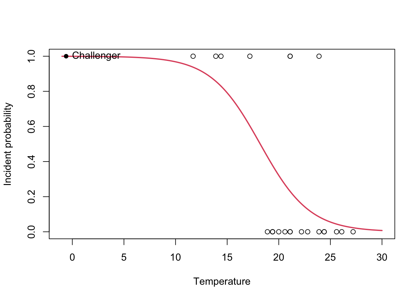

The exponentials of the estimated coefficients are:

• $e^{\hat\beta_0}=1965.974$. This means that, when the temperature is zero, the fitted odds is $1965.974$, so the probability of having an incident ($Y=1$) is $1965.974$ times larger than the probability of not having an incident ($Y=0$). In other words, the probability of having an incident at temperature zero is $\frac{1965.974}{1965.974+1}=0.999$.
• $e^{\hat\beta_1}=0.659$. This means that each Celsius degree increment in the temperature multiplies the fitted odds by a factor of $0.659\approx\frac{2}{3}$, hence reducing it.

The estimation of $\boldsymbol{\beta}=(\beta_0,\beta_1,\ldots,\beta_k)$ from a sample $(\mathbf{X}_{1},Y_1),\ldots,(\mathbf{X}_{n},Y_n)$ is different than in linear regression. It is not based on minimizing the RSS but on the principle of Maximum Likelihood Estimation (MLE). MLE is based on the following leitmotiv: what are the coefficients $\boldsymbol{\beta}$ that make the sample more likely? Or in other words, what coefficients make the model more probable, based on the sample. Since $Y_i\sim \mathrm{Ber}(p(\mathbf{X}_i))$, $i=1,\ldots,n$, the likelihood of $\boldsymbol{\beta}$ is $$\begin{align} \text{lik}(\boldsymbol{\beta})=\prod_{i=1}^np(\mathbf{X}_i)^{Y_i}(1-p(\mathbf{X}_i))^{1-Y_i}.\tag{4.8} \end{align}$$ $\text{lik}(\boldsymbol{\beta})$ is the probability of the data based on the model. Therefore, it is a number between $0$ and $1$. Its detailed interpretation is the following:

• $\prod_{i=1}^n$ appears because the sample elements are assumed to be independent and we are computing the probability of observing the whole sample $(\mathbf{X}_{1},Y_1),\ldots,(\mathbf{X}_{n},Y_n)$. This probability is equal to the product of the probabilities of observing each $(\mathbf{X}_{i},Y_i)$.
• $p(\mathbf{X}_i)^{Y_i}(1-p(\mathbf{X}_i))^{1-Y_i}$ is the probability of observing $(\mathbf{X}_{i},Y_i)$, as given by (4.3). Remember that $p$ depends on $\boldsymbol{\beta}$ due to (4.4).

Usually, the log-likelihood is considered instead of the likelihood for stability reasons – the estimates obtained are exactly the same and are $$\hat{\boldsymbol{\beta}}=\arg\max_{\boldsymbol{\beta}\in\mathbb{R}^{k+1}}\log \text{lik}(\boldsymbol{\beta}).$$ Unfortunately, due to the non-linearity of the optimization problem there are no explicit expressions for $\hat{\boldsymbol{\beta}}$. These have to be obtained numerically by means of an iterative procedure (the number of iterations required is printed in the output of summary). In low sample situations with perfect classification, the iterative procedure may not converge.

Figure 4.6 shows how the log-likelihood changes with respect to the values for $(\beta_0,\beta_1)$ in three data patterns.

Figure 4.6: The logistic regression fit and its dependence on $\beta_0$ (horizontal displacement) and $\beta_1$ (steepness of the curve). Recall the effect of the sign of $\beta_1$ in the curve: if positive, the logistic curve has an ‘s’ form; if negative, the form is a reflected ‘s.’ Application also available here.

The data of the illustration has been generated with the following code:

# Data
set.seed(34567)
x <- rnorm(50, sd = 1.5)
y1 <- -0.5 + 3 * x
y2 <- 0.5 - 2 * x
y3 <- -2 + 5 * x
y1 <- rbinom(50, size = 1, prob = 1 / (1 + exp(-y1)))
y2 <- rbinom(50, size = 1, prob = 1 / (1 + exp(-y2)))
y3 <- rbinom(50, size = 1, prob = 1 / (1 + exp(-y3)))

# Data
dataMle <- data.frame(x = x, y1 = y1, y2 = y2, y3 = y3)

Let’s check that indeed the coefficients given by glm are the ones that maximize the likelihood given in the animation of Figure 4.6. We do so for y ~ x1.

mod <- glm(y1 ~ x, family = "binomial", data = dataMle)
mod$coefficients
## (Intercept)           x 
##  -0.1691947   2.4281626

For the regressions y ~ x2 and y ~ x3, do the following:

• Check that the true $\boldsymbol{\beta}$ is close to maximizing the likelihood computed in Figure 4.6.
• Plot the fitted logistic curve and compare it with the one in Figure 4.6.

In linear regression we relied on least squares estimation, in other words, the minimization of the RSS. Why do we need MLE in logistic regression and not least squares? The answer is two-fold:

1. MLE is asymptotically optimal when estimating unknown parameters in a model. That means that when the sample size $n$ is large, it is guaranteed to perform better than any other estimation method. Therefore, considering a least squares approach for logistic regression will result in suboptimal estimates.
2. In multiple linear regression, due to the normality assumption, MLE and least squares estimation coincide. So MLE is hidden under the form of the least squares, which is a more intuitive estimation procedure. Indeed, the maximized likelihood $\text{lik}(\hat{\boldsymbol{\beta}})$ in the linear model and the RSS are intimately related.

As in the linear model, the inclusion of a new predictor changes the coefficient estimates of the logistic model.

---

29. Recall that the result of a bet is binary: you either win or lose the bet.↩︎