5.1 Examples and applications
5.1.1 Case study: Employment in European countries in the late 70s
The purpose of this case study, motivated by Hand et al. (1994) and Bartholomew et al. (2008), is to reveal the structure of the job market and economy in different developed countries. The final aim is to have a meaningful and rigorous plot that is able to show the most important features of the countries in a concise form.
The dataset eurojob (download) contains the data employed in this case study. It contains the percentage of workforce employed in 1979 in 9 industries for 26 European countries. The industries measured are:
- Agriculture (
Agr) - Mining (
Min) - Manufacturing (
Man) - Power supply industries
(Pow) - Construction (
Con) - Service industries (
Ser) - Finance (
Fin) - Social and personal services (
Soc) - Transport and communications (
Tra)
If the dataset is imported into R and the case names are set as Country (important in order to have only numerical variables), then the data should look like this:
| Country | Agr | Min | Man | Pow | Con | Ser | Fin | Soc | Tra |
|---|---|---|---|---|---|---|---|---|---|
| Belgium | 3.3 | 0.9 | 27.6 | 0.9 | 8.2 | 19.1 | 6.2 | 26.6 | 7.2 |
| Denmark | 9.2 | 0.1 | 21.8 | 0.6 | 8.3 | 14.6 | 6.5 | 32.2 | 7.1 |
| France | 10.8 | 0.8 | 27.5 | 0.9 | 8.9 | 16.8 | 6.0 | 22.6 | 5.7 |
| WGerm | 6.7 | 1.3 | 35.8 | 0.9 | 7.3 | 14.4 | 5.0 | 22.3 | 6.1 |
| Ireland | 23.2 | 1.0 | 20.7 | 1.3 | 7.5 | 16.8 | 2.8 | 20.8 | 6.1 |
| Italy | 15.9 | 0.6 | 27.6 | 0.5 | 10.0 | 18.1 | 1.6 | 20.1 | 5.7 |
| Luxem | 7.7 | 3.1 | 30.8 | 0.8 | 9.2 | 18.5 | 4.6 | 19.2 | 6.2 |
| Nether | 6.3 | 0.1 | 22.5 | 1.0 | 9.9 | 18.0 | 6.8 | 28.5 | 6.8 |
| UK | 2.7 | 1.4 | 30.2 | 1.4 | 6.9 | 16.9 | 5.7 | 28.3 | 6.4 |
| Austria | 12.7 | 1.1 | 30.2 | 1.4 | 9.0 | 16.8 | 4.9 | 16.8 | 7.0 |
| Finland | 13.0 | 0.4 | 25.9 | 1.3 | 7.4 | 14.7 | 5.5 | 24.3 | 7.6 |
| Greece | 41.4 | 0.6 | 17.6 | 0.6 | 8.1 | 11.5 | 2.4 | 11.0 | 6.7 |
| Norway | 9.0 | 0.5 | 22.4 | 0.8 | 8.6 | 16.9 | 4.7 | 27.6 | 9.4 |
| Portugal | 27.8 | 0.3 | 24.5 | 0.6 | 8.4 | 13.3 | 2.7 | 16.7 | 5.7 |
| Spain | 22.9 | 0.8 | 28.5 | 0.7 | 11.5 | 9.7 | 8.5 | 11.8 | 5.5 |
| Sweden | 6.1 | 0.4 | 25.9 | 0.8 | 7.2 | 14.4 | 6.0 | 32.4 | 6.8 |
| Switz | 7.7 | 0.2 | 37.8 | 0.8 | 9.5 | 17.5 | 5.3 | 15.4 | 5.7 |
| Turkey | 66.8 | 0.7 | 7.9 | 0.1 | 2.8 | 5.2 | 1.1 | 11.9 | 3.2 |
| Bulgaria | 23.6 | 1.9 | 32.3 | 0.6 | 7.9 | 8.0 | 0.7 | 18.2 | 6.7 |
| Czech | 16.5 | 2.9 | 35.5 | 1.2 | 8.7 | 9.2 | 0.9 | 17.9 | 7.0 |
| EGerm | 4.2 | 2.9 | 41.2 | 1.3 | 7.6 | 11.2 | 1.2 | 22.1 | 8.4 |
| Hungary | 21.7 | 3.1 | 29.6 | 1.9 | 8.2 | 9.4 | 0.9 | 17.2 | 8.0 |
| Poland | 31.1 | 2.5 | 25.7 | 0.9 | 8.4 | 7.5 | 0.9 | 16.1 | 6.9 |
| Romania | 34.7 | 2.1 | 30.1 | 0.6 | 8.7 | 5.9 | 1.3 | 11.7 | 5.0 |
| USSR | 23.7 | 1.4 | 25.8 | 0.6 | 9.2 | 6.1 | 0.5 | 23.6 | 9.3 |
| Yugoslavia | 48.7 | 1.5 | 16.8 | 1.1 | 4.9 | 6.4 | 11.3 | 5.3 | 4.0 |
So far, we know how to compute summaries for each variable, and how to quantify and visualize relations between variables with the correlation matrix and the scatterplot matrix. But even for a moderate number of variables like this, their results are hard to process.
# Summary of the data - marginal
summary(eurojob)
##       Agr             Min             Man             Pow
##  Min.   : 2.70   Min.   :0.100   Min.   : 7.90   Min.   :0.1000
##  1st Qu.: 7.70   1st Qu.:0.525   1st Qu.:23.00   1st Qu.:0.6000
##  Median :14.45   Median :0.950   Median :27.55   Median :0.8500
##  Mean   :19.13   Mean   :1.254   Mean   :27.01   Mean   :0.9077
##  3rd Qu.:23.68   3rd Qu.:1.800   3rd Qu.:30.20   3rd Qu.:1.1750
##  Max.   :66.80   Max.   :3.100   Max.   :41.20   Max.   :1.9000
##       Con              Ser             Fin              Soc
##  Min.   : 2.800   Min.   : 5.20   Min.   : 0.500   Min.   : 5.30
##  1st Qu.: 7.525   1st Qu.: 9.25   1st Qu.: 1.225   1st Qu.:16.25
##  Median : 8.350   Median :14.40   Median : 4.650   Median :19.65
##  Mean   : 8.165   Mean   :12.96   Mean   : 4.000   Mean   :20.02
##  3rd Qu.: 8.975   3rd Qu.:16.88   3rd Qu.: 5.925   3rd Qu.:24.12
##  Max.   :11.500   Max.   :19.10   Max.   :11.300   Max.   :32.40
##       Tra
##  Min.   :3.200
##  1st Qu.:5.700
##  Median :6.700
##  Mean   :6.546
##  3rd Qu.:7.075
##  Max.   :9.400

# Correlation matrix
cor(eurojob)
##             Agr         Min        Man         Pow         Con        Ser
## Agr  1.00000000  0.03579884 -0.6710976 -0.40005113 -0.53832522 -0.7369805
## Min  0.03579884  1.00000000  0.4451960  0.40545524 -0.02559781 -0.3965646
## Man -0.67109759  0.44519601  1.0000000  0.38534593  0.49447949  0.2038263
## Pow -0.40005113  0.40545524  0.3853459  1.00000000  0.05988883  0.2019066
## Con -0.53832522 -0.02559781  0.4944795  0.05988883  1.00000000  0.3560216
## Ser -0.73698054 -0.39656456  0.2038263  0.20190661  0.35602160  1.0000000
## Fin -0.21983645 -0.44268311 -0.1558288  0.10986158  0.01628255  0.3655553
## Soc -0.74679001 -0.28101212  0.1541714  0.13241132  0.15824309  0.5721728
## Tra -0.56492047  0.15662892  0.3506925  0.37523116  0.38766214  0.1875543
##             Fin        Soc        Tra
## Agr -0.21983645 -0.7467900 -0.5649205
## Min -0.44268311 -0.2810121  0.1566289
## Man -0.15582884  0.1541714  0.3506925
## Pow  0.10986158  0.1324113  0.3752312
## Con  0.01628255  0.1582431  0.3876621
## Ser  0.36555529  0.5721728  0.1875543
## Fin  1.00000000  0.1076403 -0.2459257
## Soc  0.10764028  1.0000000  0.5678669
## Tra -0.24592567  0.5678669  1.0000000

# Scatterplot matrix
scatterplotMatrix(eurojob, reg.line = lm, smooth = FALSE, spread = FALSE,
                  span = 0.5, ellipse = FALSE, levels = c(.5, .9), id.n = 0,
                  diagonal = 'histogram')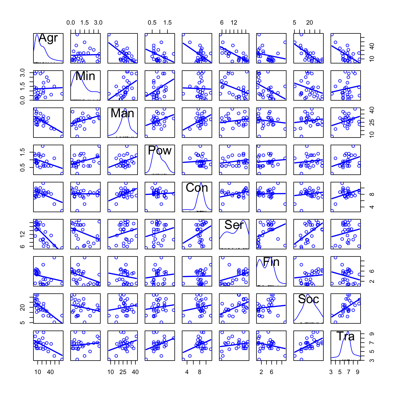
We definitely need a way of visualizing and quantifying the relations between variables for a moderate to large amount of variables. PCA will be a handy way. In a nutshell, what PCA does is:
- Takes the data for the variables \(X_1,\ldots,X_k\).
- Using this data, looks for new variables \(\text{PC}_1,\ldots \text{PC}_k\) such that:
- \(\text{PC}_j\) is a linear combination of \(X_1,\ldots,X_k\), \(1\leq j\leq k\). This is, \(\text{PC}_j=a_{1j}X_1+a_{2j}X_2+\cdots+a_{kj}X_k\).
- \(\text{PC}_1,\ldots \text{PC}_k\) are sorted decreasingly in terms of variance. Hence \(\text{PC}_j\) has more variance than \(\text{PC}_{j+1}\), \(1\leq j\leq k-1\),
- \(\text{PC}_{j_1}\) and \(\text{PC}_{j_2}\) are uncorrelated, for \(j_1\neq j_2\).
- \(\text{PC}_1,\ldots \text{PC}_k\) have the same information, measured in terms of total variance, as \(X_1,\ldots,X_k\).
- Produces three key objects:
- Variances of the PCs. They are sorted decreasingly and give an idea of which PCs are contain most of the information of the data (the ones with more variance).
- Weights of the variables in the PCs. They give the interpretation of the PCs in terms of the original variables, as they are the coefficients of the linear combination. The weights of the variables \(X_1,\ldots,X_k\) on the PC\(_j\), \(a_{1j},\ldots,a_{kj}\), are normalized: \(a_{1j}^2+\cdots+a_{kj}^2=1\), \(j=1,\ldots,k\). In R, they are called
loadings. - Scores of the data in the PCs: this is the data with \(\text{PC}_1,\ldots \text{PC}_k\) variables instead of \(X_1,\ldots,X_k\). The scores are uncorrelated. Useful for knowing which PCs have more effect on a certain observation.
Hence, PCA rearranges our variables in an information-equivalent, but more convenient, layout where the variables are sorted according to the amount of information they are able to explain. From this position, the next step is clear: stick only with a limited number of PCs such that they explain most of the information (e.g., 70% of the total variance) and do dimension reduction. The effectiveness of PCA in practice varies from the structure present in the dataset. For example, in the case of highly dependent data, it could explain more than the 90% of variability of a dataset with tens of variables with just two PCs.
Let’s see how to compute a full PCA in R.
# The main function - use cor = TRUE to avoid scale distortions
pca <- princomp(eurojob, cor = TRUE)

# What is inside?
str(pca)
## List of 7
##  $ sdev    : Named num [1:9] 1.867 1.46 1.048 0.997 0.737 ...
##   ..- attr(*, "names")= chr [1:9] "Comp.1" "Comp.2" "Comp.3" "Comp.4" ...
##  $ loadings: 'loadings' num [1:9, 1:9] 0.52379 0.00132 -0.3475 -0.25572 -0.32518 ...
##   ..- attr(*, "dimnames")=List of 2
##   .. ..$ : chr [1:9] "Agr" "Min" "Man" "Pow" ...
##   .. ..$ : chr [1:9] "Comp.1" "Comp.2" "Comp.3" "Comp.4" ...
##  $ center  : Named num [1:9] 19.131 1.254 27.008 0.908 8.165 ...
##   ..- attr(*, "names")= chr [1:9] "Agr" "Min" "Man" "Pow" ...
##  $ scale   : Named num [1:9] 15.245 0.951 6.872 0.369 1.614 ...
##   ..- attr(*, "names")= chr [1:9] "Agr" "Min" "Man" "Pow" ...
##  $ n.obs   : int 26
##  $ scores  : num [1:26, 1:9] -1.71 -0.953 -0.755 -0.853 0.104 ...
##   ..- attr(*, "dimnames")=List of 2
##   .. ..$ : chr [1:26] "Belgium" "Denmark" "France" "WGerm" ...
##   .. ..$ : chr [1:9] "Comp.1" "Comp.2" "Comp.3" "Comp.4" ...
##  $ call    : language princomp(x = eurojob, cor = TRUE)
##  - attr(*, "class")= chr "princomp"

# The standard deviation of each PC
pca$sdev
##      Comp.1      Comp.2      Comp.3      Comp.4      Comp.5      Comp.6
## 1.867391569 1.459511268 1.048311791 0.997237674 0.737033056 0.619215363
##      Comp.7      Comp.8      Comp.9
## 0.475135828 0.369851221 0.006754636

# Weights: the expression of the original variables in the PCs
# E.g. Agr = -0.524 * PC1 + 0.213 * PC5 - 0.152 * PC6 + 0.806 * PC9
# And also: PC1 = -0.524 * Agr + 0.347 * Man + 0256 * Pow + 0.325 * Con + ...
# (Because the matrix is orthogonal, so the transpose is the inverse)
pca$loadings
##
## Loadings:
##     Comp.1 Comp.2 Comp.3 Comp.4 Comp.5 Comp.6 Comp.7 Comp.8 Comp.9
## Agr  0.524                       0.213  0.153                0.806
## Min         0.618 -0.201        -0.164 -0.101 -0.726
## Man -0.347  0.355 -0.150 -0.346 -0.385 -0.288  0.479  0.126  0.366
## Pow -0.256  0.261 -0.561  0.393  0.295  0.357  0.256 -0.341
## Con -0.325         0.153 -0.668  0.472  0.130 -0.221 -0.356
## Ser -0.379 -0.350 -0.115        -0.284  0.615 -0.229  0.388  0.238
## Fin        -0.454 -0.587         0.280 -0.526 -0.187  0.174  0.145
## Soc -0.387 -0.222  0.312  0.412 -0.220 -0.263 -0.191 -0.506  0.351
## Tra -0.367  0.203  0.375  0.314  0.513 -0.124         0.545
##
##                Comp.1 Comp.2 Comp.3 Comp.4 Comp.5 Comp.6 Comp.7 Comp.8 Comp.9
## SS loadings     1.000  1.000  1.000  1.000  1.000  1.000  1.000  1.000  1.000
## Proportion Var  0.111  0.111  0.111  0.111  0.111  0.111  0.111  0.111  0.111
## Cumulative Var  0.111  0.222  0.333  0.444  0.556  0.667  0.778  0.889  1.000

# Scores of the data on the PCs: how is the data re-expressed into PCs
head(pca$scores, 10)
##             Comp.1      Comp.2      Comp.3      Comp.4      Comp.5      Comp.6
## Belgium -1.7104977 -1.22179120 -0.11476476  0.33949201 -0.32453569 -0.04725409
## Denmark -0.9529022 -2.12778495  0.95072216  0.59394893  0.10266111 -0.82730228
## France  -0.7546295 -1.12120754 -0.49795370 -0.50032910 -0.29971876  0.11580705
## WGerm   -0.8525525 -0.01137659 -0.57952679 -0.11046984 -1.16522683 -0.61809939
## Ireland  0.1035018 -0.41398717 -0.38404787  0.92666396  0.01522133  1.42419990
## Italy   -0.3754065 -0.76954739  1.06059786 -1.47723127 -0.64518265  1.00210439
## Luxem   -1.0594424  0.75582714 -0.65147987 -0.83515611 -0.86593673  0.21879618
## Nether  -1.6882170 -2.00484484  0.06374194 -0.02351427  0.63517966  0.21197502
## UK      -1.6304491 -0.37312967 -1.14090318  1.26687863 -0.81292541 -0.03605094
## Austria -1.1764484  0.14310057 -1.04336386 -0.15774745  0.52098078  0.80190706
##              Comp.7     Comp.8        Comp.9
## Belgium -0.34008766  0.4030352 -0.0010904043
## Denmark -0.30292281 -0.3518357  0.0156187715
## France  -0.18547802 -0.2661924 -0.0005074307
## WGerm    0.44455923  0.1944841 -0.0065393717
## Ireland -0.03704285 -0.3340389  0.0108793301
## Italy   -0.14178212 -0.1302796  0.0056017552
## Luxem   -1.69417817  0.5473283  0.0034530991
## Nether  -0.30339781 -0.5906297 -0.0109314745
## UK       0.04128463 -0.3485948 -0.0054775709
## Austria  0.41503736  0.2150993 -0.0028164222

# Scatterplot matrix of the scores - they are uncorrelated!
scatterplotMatrix(pca$scores, reg.line = lm, smooth = FALSE, spread = FALSE,
                  span = 0.5, ellipse = FALSE, levels = c(.5, .9), id.n = 0,
                  diagonal = 'histogram')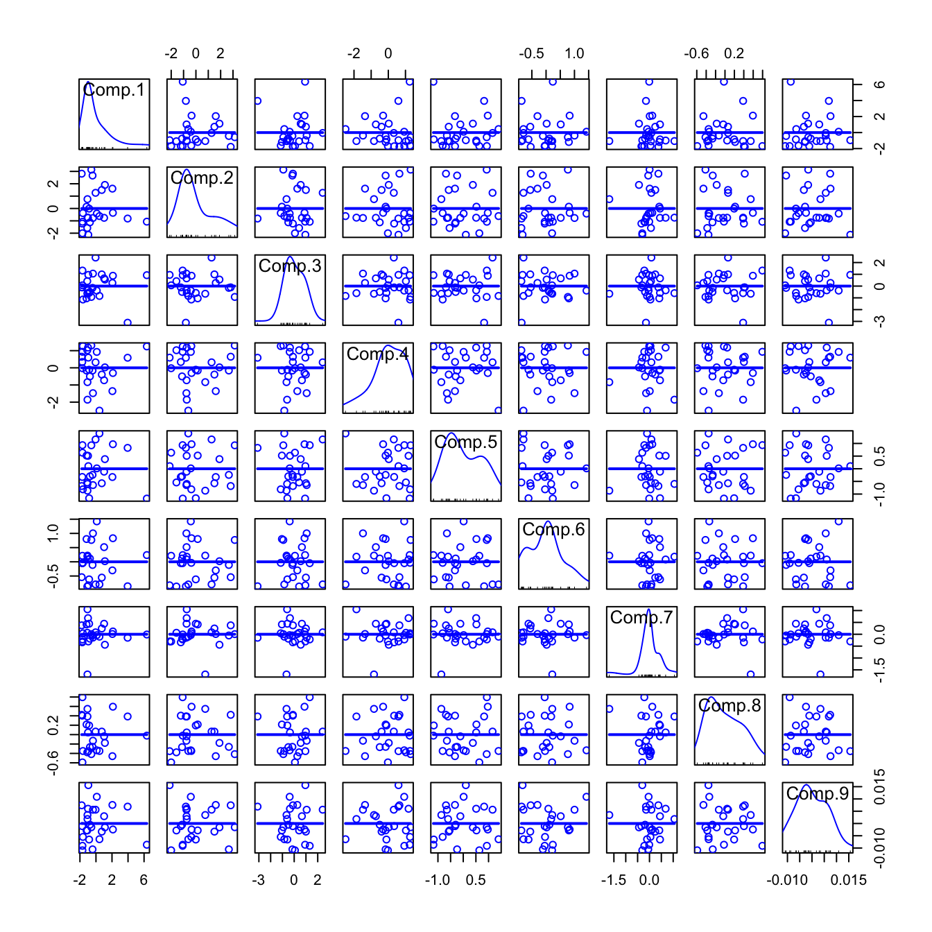
# Means of the variables - before PCA the variables are centered
pca$center
##        Agr        Min        Man        Pow        Con        Ser        Fin
## 19.1307692  1.2538462 27.0076923  0.9076923  8.1653846 12.9576923  4.0000000
##        Soc        Tra
## 20.0230769  6.5461538

# Rescaling done to each variable
# - if cor = FALSE (default), a vector of ones
# - if cor = TRUE, a vector with the standard deviations of the variables
pca$scale
##        Agr        Min        Man        Pow        Con        Ser        Fin
## 15.2446654  0.9512060  6.8716767  0.3689101  1.6136300  4.4864045  2.7520622
##        Soc        Tra
##  6.6969171  1.3644471

# Summary of the importance of components - the third row is key
summary(pca)
## Importance of components:
##                           Comp.1    Comp.2    Comp.3    Comp.4     Comp.5
## Standard deviation     1.8673916 1.4595113 1.0483118 0.9972377 0.73703306
## Proportion of Variance 0.3874613 0.2366859 0.1221064 0.1104981 0.06035753
## Cumulative Proportion  0.3874613 0.6241472 0.7462536 0.8567517 0.91710919
##                            Comp.6     Comp.7     Comp.8       Comp.9
## Standard deviation     0.61921536 0.47513583 0.36985122 6.754636e-03
## Proportion of Variance 0.04260307 0.02508378 0.01519888 5.069456e-06
## Cumulative Proportion  0.95971227 0.98479605 0.99999493 1.000000e+00

# Scree plot - the variance of each component
plot(pca)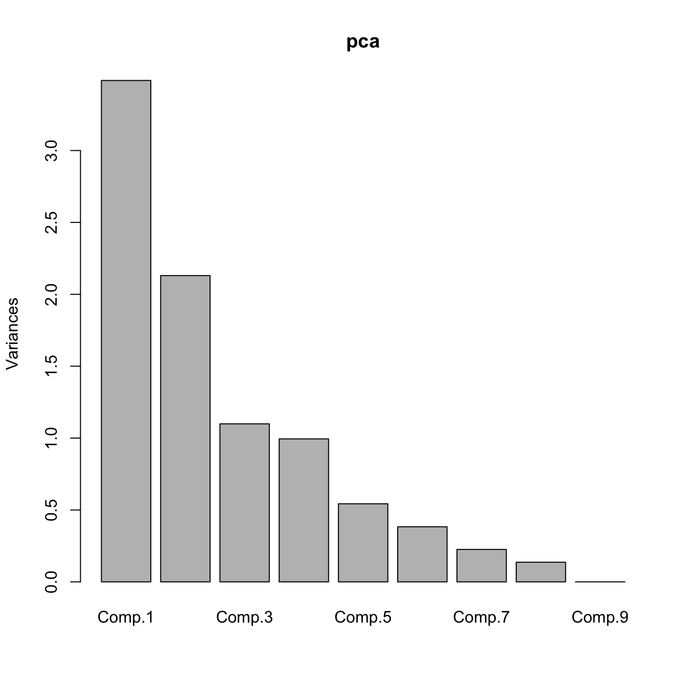
# With connected lines - useful for looking for the "elbow"
plot(pca, type = "l")
# PC1 and PC2
pca$loadings[, 1:2]
##           Comp.1      Comp.2
## Agr  0.523790989  0.05359389
## Min  0.001323458  0.61780714
## Man -0.347495131  0.35505360
## Pow -0.255716182  0.26109606
## Con -0.325179319  0.05128845
## Ser -0.378919663 -0.35017206
## Fin -0.074373583 -0.45369785
## Soc -0.387408806 -0.22152120
## Tra -0.366822713  0.20259185
PCA produces uncorrelated variables from the original set \(X_1,\ldots,X_k\). This implies that:
- The PCs are uncorrelated, but not independent (uncorrelated does not imply independent).
- An uncorrelated or independent variable in \(X_1,\ldots,X_k\) will get a PC only associated to it. In the extreme case where all the \(X_1,\ldots,X_k\) are uncorrelated, these coincide with the PCs (up to sign flips).
Based on the weights of the variables on the PCs, we can extract the following interpretation:
- PC1 is roughly a linear combination of
Agr, with negative weight, and (Man,Pow,Con,Ser,Soc,Tra), with positive weights. So it can be interpreted as an indicator of the kind of economy of the country: agricultural (negative values) or industrial (positive values). - PC2 has negative weights on (
Min,Man,Pow,Tra) and positive weights in (Ser,Fin,Soc). It can be interpreted as the contrast between relatively large or small service sectors. So it tends to be negative in communist countries and positive in capitalist countries.
The interpretation of the PCs involves inspecting the weights and interpreting the linear combination of the original variables, which might be separating between two clear characteristics of the data
To conclude, let’s see how we can represent our original data into a plot called biplot that summarizes all the analysis for two PCs.
# Biplot - plot together the scores for PC1 and PC2 and the
# variables expressed in terms of PC1 and PC2
biplot(pca)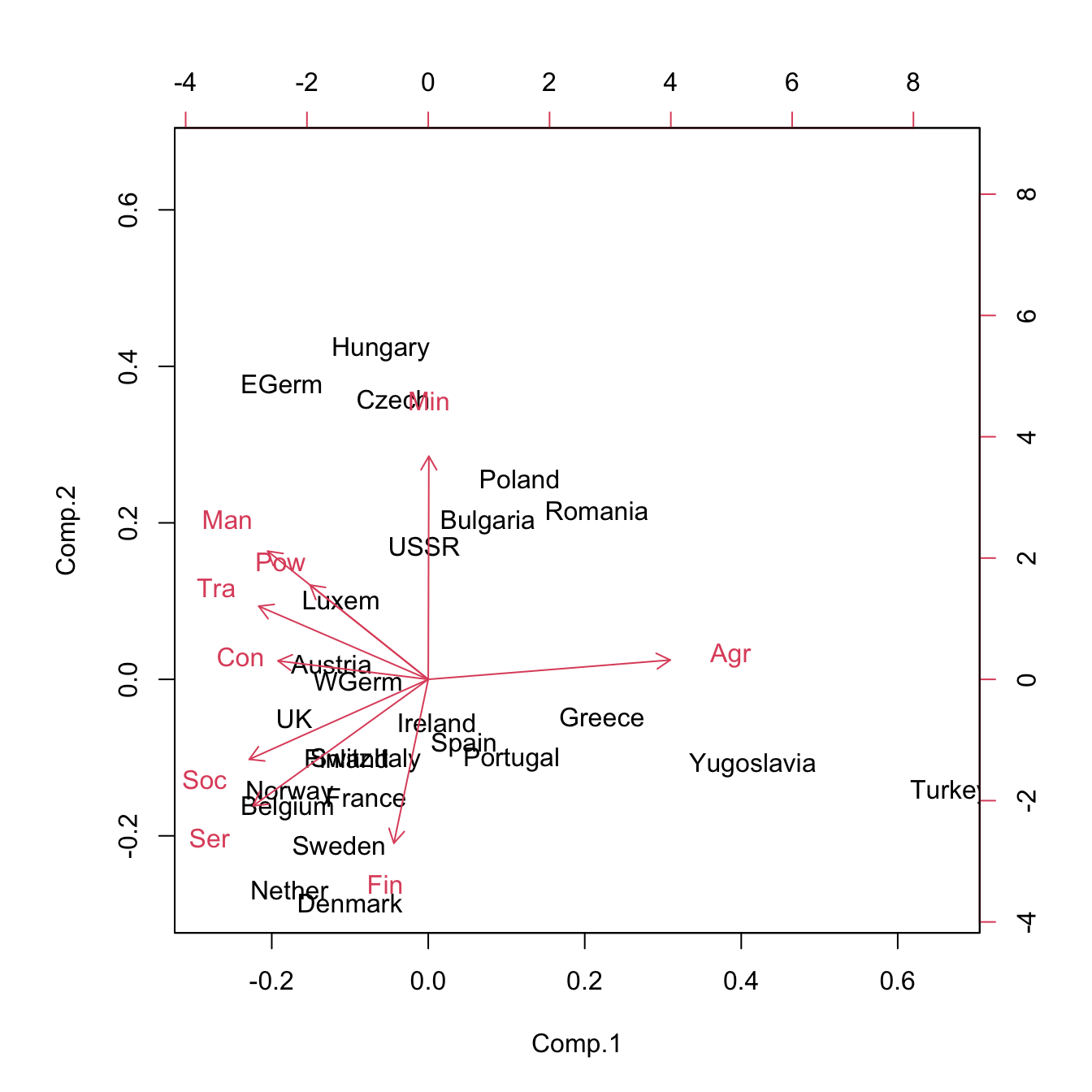
5.1.2 Case studies: Analysis of USArrests, USJudgeRatings and La Liga 2015/2016 metrics
The selection of the number of PCs and their interpretation though the weights and biplots are key aspects in a successful application of PCA. In this section we will see examples of both points through the datasets USArrests, USJudgeRatings and La Liga 2015/2016 (download).
The selection of the number of components \(l\), \(1\leq l\leq k\)32, is a tricky problem without a unique and well-established criterion for what is the best number of components. The reason is that selecting the number of PCs is a trade-off between the variance of the original data that we want to explain and the price we want to pay in terms of a more complex dataset. Obviously, except for particular cases33, none of the extreme situations \(l=1\) (potential low explained variance) or \(l=k\) (same number of PCs as the original data – no dimension reduction) is desirable.
There are several heuristic rules in order to determine the number of components:
- Select \(l\) up to a threshold of the percentage of variance explained, such as \(70\%\) or \(80\%\). We do so by looking into the third row of the
summary(...)of a PCA. - Plot the variances of the PCs and look for an “elbow” in the graph whose location gives \(l\). Ideally, this elbow appears at the PC for which the next PC variances are almost similar and notably smaller when compared with the first ones. Use
plot(..., type = "l")for creating the plot. - Select \(l\) based on the threshold of the individual variance of each component. For example, select only the PCs with larger variance than the mean of the variances of all the PCs. If we are working with standardized variables (
cor = TRUE), this equals to taking the PCs with standard deviation larger than one. We do so by looking into the first row of thesummary(...)of a PCA.
In addition to these three heuristics, in practice we might apply a justified bias towards:
- \(l=1,2\), since these are the ones that allow to have a simple graphical representation of the data. Even if the variability explained by the \(l\) PCs is low (lower than \(50\%\)), these graphical representations are usually insightful. \(l=3\) is preferred as a second option since its graphical representation is more cumbersome (see the end of this section).
- \(l\)’s such that they yield interpretable PCs. Interpreting PCs is not so straightforward as interpreting the original variables. Furthermore, it becomes more difficult the larger the index of the PC is, since it explains less information of the data.
Let’s see these heuristics in practice with the USArrests dataset (arrest statistics and population of US states).
# Load data
data(USArrests)
# Snapshot of the data
head(USArrests)
## Murder Assault UrbanPop Rape
## Alabama 13.2 236 58 21.2
## Alaska 10.0 263 48 44.5
## Arizona 8.1 294 80 31.0
## Arkansas 8.8 190 50 19.5
## California 9.0 276 91 40.6
## Colorado 7.9 204 78 38.7
# PCA
pcaUSArrests <- princomp(USArrests, cor = TRUE)
summary(pcaUSArrests)
## Importance of components:
## Comp.1 Comp.2 Comp.3 Comp.4
## Standard deviation 1.5748783 0.9948694 0.5971291 0.41644938
## Proportion of Variance 0.6200604 0.2474413 0.0891408 0.04335752
## Cumulative Proportion 0.6200604 0.8675017 0.9566425 1.00000000
# Plot of variances (screeplot)
plot(pcaUSArrests, type = "l")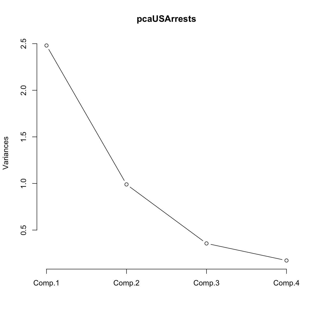 The selections of \(l\) for this PCA, based on the previous heuristics, are:
- \(l=2\), since it explains the \(86\%\) of the variance and \(l=1\) only the \(62\%\).
- \(l=2\), since from \(l=2\) onward the variances are very similar.
- \(l=1\), since the \(\text{PC}_2\) has standard deviation smaller than \(1\) (limit case).
- \(l=2\) is fine, it can be easily represented graphically.
- \(l=2\) is fine, both components are interpretable, as we will see later.
Therefore, we can conclude that \(l=2\) PCs is a good compromise for representing the USArrests dataset.
Let’s see what happens for the USJudgeRatings dataset (lawyers’ ratings of US Superior Court judges).
# Load data
data(USJudgeRatings)
# Snapshot of the data
head(USJudgeRatings)
## CONT INTG DMNR DILG CFMG DECI PREP FAMI ORAL WRIT PHYS RTEN
## AARONSON,L.H. 5.7 7.9 7.7 7.3 7.1 7.4 7.1 7.1 7.1 7.0 8.3 7.8
## ALEXANDER,J.M. 6.8 8.9 8.8 8.5 7.8 8.1 8.0 8.0 7.8 7.9 8.5 8.7
## ARMENTANO,A.J. 7.2 8.1 7.8 7.8 7.5 7.6 7.5 7.5 7.3 7.4 7.9 7.8
## BERDON,R.I. 6.8 8.8 8.5 8.8 8.3 8.5 8.7 8.7 8.4 8.5 8.8 8.7
## BRACKEN,J.J. 7.3 6.4 4.3 6.5 6.0 6.2 5.7 5.7 5.1 5.3 5.5 4.8
## BURNS,E.B. 6.2 8.8 8.7 8.5 7.9 8.0 8.1 8.0 8.0 8.0 8.6 8.6
# PCA
pcaUSJudgeRatings <- princomp(USJudgeRatings, cor = TRUE)
summary(pcaUSJudgeRatings)
## Importance of components:
## Comp.1 Comp.2 Comp.3 Comp.4 Comp.5
## Standard deviation 3.1833165 1.05078398 0.5769763 0.50383231 0.290607615
## Proportion of Variance 0.8444586 0.09201225 0.0277418 0.02115392 0.007037732
## Cumulative Proportion 0.8444586 0.93647089 0.9642127 0.98536661 0.992404341
## Comp.6 Comp.7 Comp.8 Comp.9
## Standard deviation 0.193095982 0.140295449 0.124158319 0.0885069038
## Proportion of Variance 0.003107172 0.001640234 0.001284607 0.0006527893
## Cumulative Proportion 0.995511513 0.997151747 0.998436354 0.9990891437
## Comp.10 Comp.11 Comp.12
## Standard deviation 0.0749114592 0.0570804224 0.0453913429
## Proportion of Variance 0.0004676439 0.0002715146 0.0001716978
## Cumulative Proportion 0.9995567876 0.9998283022 1.0000000000
# Plot of variances (screeplot)
plot(pcaUSJudgeRatings, type = "l")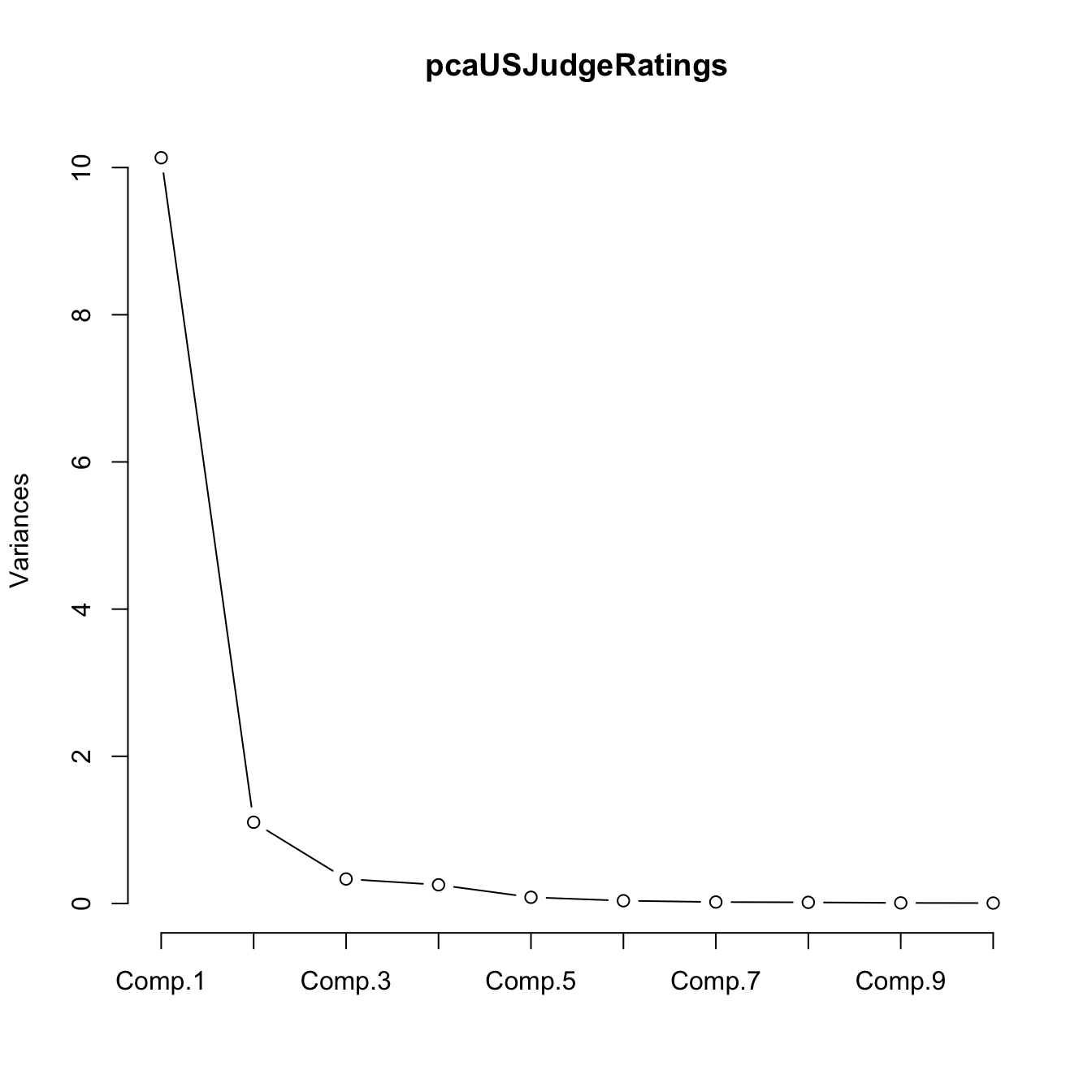 The selections of \(l\) for this PCA, based on the previous heuristics, are:
- \(l=1\), since it explains alone the \(84\%\) of the variance.
- \(l=1\), since from \(l=1\) onward the variances are very similar compared to the first one.
- \(l=2\), since the \(\text{PC}_3\) has standard deviation smaller than \(1\).
- \(l=1,2\) are fine, they can be easily represented graphically.
- \(l=1,2\) are fine, both components are interpretable, as we will see later.
Based on the previous criteria, we can conclude that \(l=1\) PC is a reasonable compromise for representing the USJudgeRatings dataset.
We analyze now a slightly more complicated dataset. It contains the standings and team statistics for La Liga 2015/2016:
| Points | Matches | Wins | Draws | Loses | |
|---|---|---|---|---|---|
| Barcelona | 91 | 38 | 29 | 4 | 5 |
| Real Madrid | 90 | 38 | 28 | 6 | 4 |
| Atlético Madrid | 88 | 38 | 28 | 4 | 6 |
| Villarreal | 64 | 38 | 18 | 10 | 10 |
| Athletic | 62 | 38 | 18 | 8 | 12 |
| Celta | 60 | 38 | 17 | 9 | 12 |
| Sevilla | 52 | 38 | 14 | 10 | 14 |
| Málaga | 48 | 38 | 12 | 12 | 14 |
| Real Sociedad | 48 | 38 | 13 | 9 | 16 |
| Betis | 45 | 38 | 11 | 12 | 15 |
| Las Palmas | 44 | 38 | 12 | 8 | 18 |
| Valencia | 44 | 38 | 11 | 11 | 16 |
| Eibar | 43 | 38 | 11 | 10 | 17 |
| Espanyol | 43 | 38 | 12 | 7 | 19 |
| Deportivo | 42 | 38 | 8 | 18 | 12 |
| Granada | 39 | 38 | 10 | 9 | 19 |
| Sporting Gijón | 39 | 38 | 10 | 9 | 19 |
| Rayo Vallecano | 38 | 38 | 9 | 11 | 18 |
| Getafe | 36 | 38 | 9 | 9 | 20 |
| Levante | 32 | 38 | 8 | 8 | 22 |
# PCA - we remove the second variable, matches played, since it is constant
pcaLaliga <- princomp(laliga[, -2], cor = TRUE)
summary(pcaLaliga)
## Importance of components:
## Comp.1 Comp.2 Comp.3 Comp.4 Comp.5
## Standard deviation 3.4372781 1.5514051 1.14023547 0.91474383 0.85799980
## Proportion of Variance 0.6563823 0.1337143 0.07222983 0.04648646 0.04089798
## Cumulative Proportion 0.6563823 0.7900966 0.86232642 0.90881288 0.94971086
## Comp.6 Comp.7 Comp.8 Comp.9 Comp.10
## Standard deviation 0.60295746 0.4578613 0.373829925 0.327242606 0.22735805
## Proportion of Variance 0.02019765 0.0116465 0.007763823 0.005949318 0.00287176
## Cumulative Proportion 0.96990851 0.9815550 0.989318830 0.995268148 0.99813991
## Comp.11 Comp.12 Comp.13 Comp.14
## Standard deviation 0.1289704085 0.0991188181 0.0837498223 2.860411e-03
## Proportion of Variance 0.0009240759 0.0005458078 0.0003896685 4.545528e-07
## Cumulative Proportion 0.9990639840 0.9996097918 0.9999994603 9.999999e-01
## Comp.15 Comp.16 Comp.17 Comp.18
## Standard deviation 1.238298e-03 1.583337e-08 1.154388e-08 0
## Proportion of Variance 8.518782e-08 1.392753e-17 7.403399e-18 0
## Cumulative Proportion 1.000000e+00 1.000000e+00 1.000000e+00 1
# Plot of variances (screeplot)
plot(pcaLaliga, type = "l")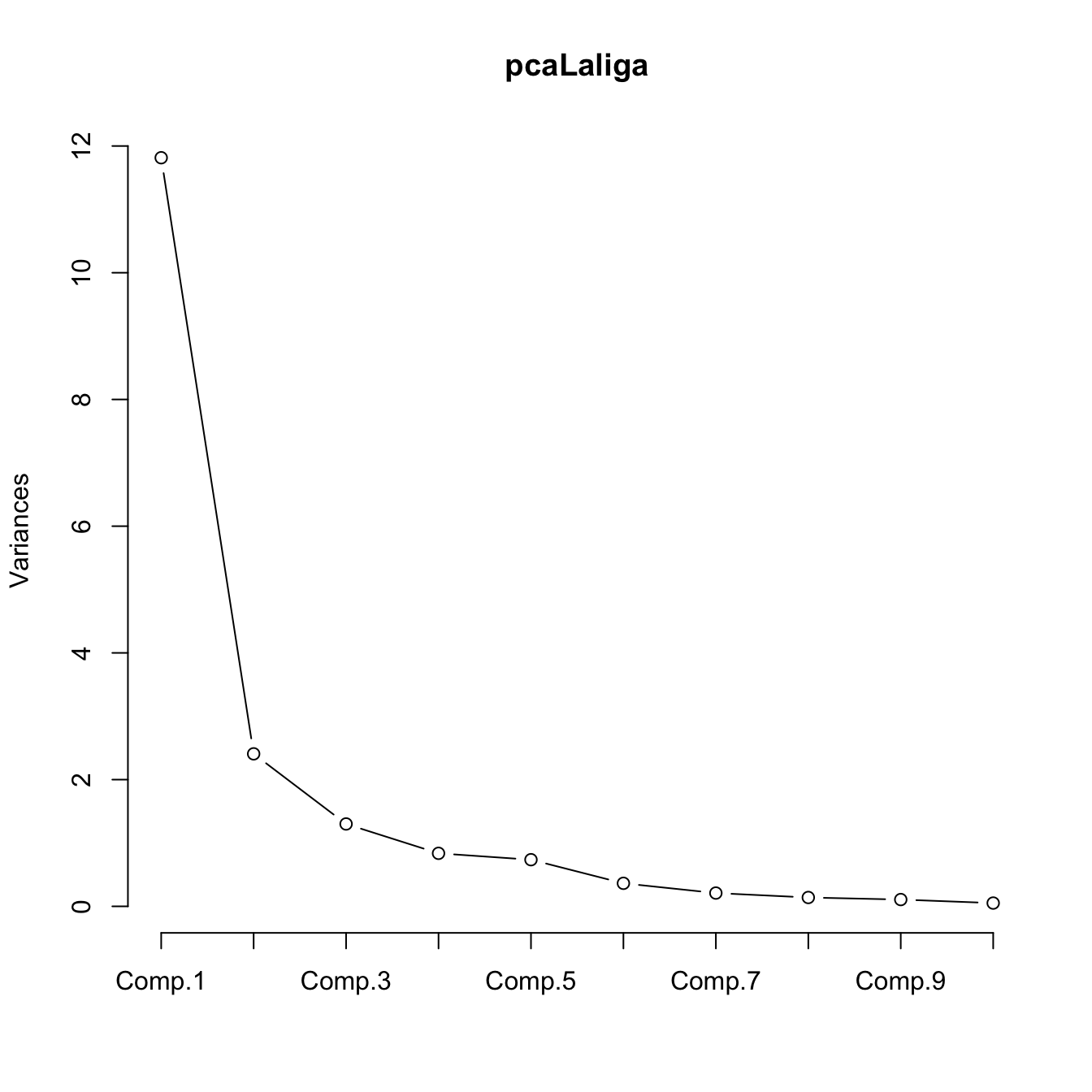 The selections of \(l\) for this PCA, based on the previous heuristics, are:
- \(l=2,3\), since they explain the \(79\%\) and \(86\%\) of the variance (it depends on the threshold of the variance, \(70\%\) or \(80\%\)).
- \(l=3\), since from \(l=1\) onward the variances are very similar compared to the first one.
- \(l=3\), since the \(\text{PC}_4\) has standard deviation smaller than \(1\).
- \(l=2\) is preferred to \(l=3\).
- \(l=1,2\) are fine, both components are interpretable, as we will see later. \(l=3\) is harder to interpret.
Based on the previous criteria, we can conclude that \(l=2\) PCs is a reasonable compromise for representing La Liga 2015/2016 dataset.
Let’s focus now on the interpretation of the PCs. In addition to the weights present in the loadings slot, biplot provides a powerful and succinct way of displaying the relevant information for \(1\leq l\leq 2\). The biplot shows:
- The scores of the data in PC1 and PC2 by points (with optional text labels, depending if there are case names). This is the representation of the data in the first two PCs.
- The variables represented in the PC1 and PC2 by the arrows. These arrows are centered at \((0, 0)\).
Let’s examine the arrow associated to the variable \(X_j\). \(X_j\) is expressed in terms of \(\text{PC}_1\) and \(\text{PC}_2\) by the weights \(a_{j1}\) and \(a_{j2}\): \[ X_j=a_{j1}\text{PC}_{1} + a_{j2}\text{PC}_{2} + \cdots + a_{jk}\text{PC}_{k}\approx a_{j1}\text{PC}_{1} + a_{j2}\text{PC}_{2}. \] \(a_{j1}\) and \(a_{j2}\) have the same sign as \(\mathrm{Cor}(X_j,\text{PC}_{1})\) and \(\mathrm{Cor}(X_j,\text{PC}_{2})\), respectively. The arrow associated to \(X_j\) is given by the segment joining \((0,0)\) and \((a_{j1},a_{j2})\). Therefore:
- If the arrow points right (\(a_{j1}>0\)), there is positive correlation between \(X_j\) and \(\text{PC}_1\). Analogous if the arrow points left.
- If the arrow is approximately vertical (\(a_{j1}\approx0\)), there is uncorrelation between \(X_j\) and \(\text{PC}_1\).
Analogously:
- If the arrow points up (\(a_{j2}>0\)), there is positive correlation between \(X_j\) and \(\text{PC}_2\). Analogous if the arrow points down.
- If the arrow is approximately horizontal (\(a_{j2}\approx0\)), there is uncorrelation between \(X_j\) and \(\text{PC}_2\).
In addition, the magnitude of the arrow informs about the correlation.
The biplot also provides the direct relation between variables, at sight of their expressions in \(\text{PC}_1\) and \(\text{PC}_2\). The angle of the arrows of variable \(X_j\) and \(X_m\) gives an approximation to the correlation between them, \(\mathrm{Cor}(X_j,X_m)\):
- If \(\text{angle}\approx 0^\circ\), the two variables are highly positively correlated.
- If \(\text{angle}\approx 90^\circ\), they are approximately uncorrelated.
- If \(\text{angle}\approx 180^\circ\), the two variables are highly negatively correlated.
The approximation to the correlation by means of the arrow angles is as good as the percentage of variance explained by \(\text{PC}_1\) and \(\text{PC}_2\).
Let see an in-depth illustration of the previous concepts for pcaUSArrests:
# Weights and biplot
pcaUSArrests$loadings
##
## Loadings:
## Comp.1 Comp.2 Comp.3 Comp.4
## Murder 0.536 0.418 0.341 0.649
## Assault 0.583 0.188 0.268 -0.743
## UrbanPop 0.278 -0.873 0.378 0.134
## Rape 0.543 -0.167 -0.818
##
## Comp.1 Comp.2 Comp.3 Comp.4
## SS loadings 1.00 1.00 1.00 1.00
## Proportion Var 0.25 0.25 0.25 0.25
## Cumulative Var 0.25 0.50 0.75 1.00biplot(pcaUSArrests)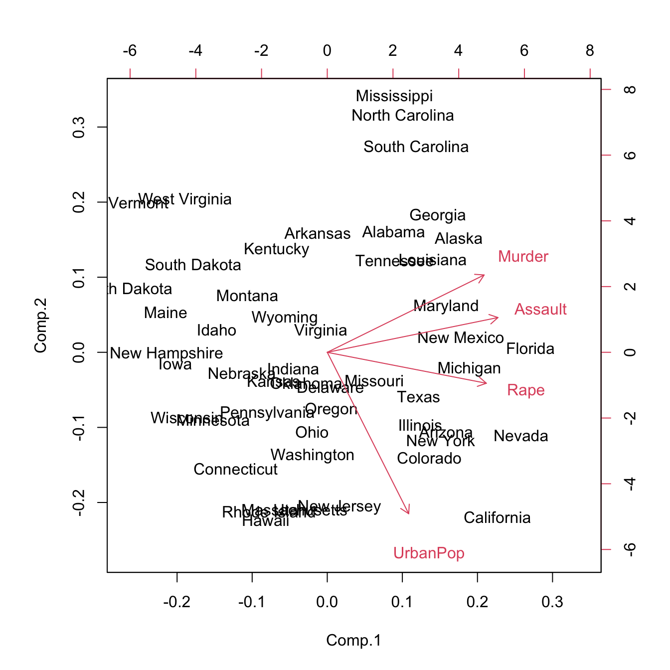 We can extract the following conclusions regarding the arrows and PCs:
Murder,AssaultandRapeare negatively correlated with \(\text{PC}_1\), which might be regarded as an indicator of the absence of crime (positive for less crimes, negative for more). The variables are highly correlated between them and the arrows are: \[\begin{align*} \vec{\text{Murder}} = (-0.536, 0.418)\\ \vec{\text{Assault}} = (-0.583, 0.188)\\ \vec{\text{Rape}} = (-0.543, -0.167) \end{align*}\]MurderandUrbanPopare approximately uncorrelated.UrbanPopis the most correlated variable with \(\text{PC}_2\) (positive for low urban population, negative for high). Its arrow is: \[\begin{align*} \vec{\text{UrbanPop}} = (-0.278 -0.873). \end{align*}\] Therefore, the biplot shows that states like Florida, South Carolina and California have high crime rate, whereas states like North Dakota or Vermont have low crime rate. California, in addition to have a high crime rate has a large urban population, whereas South Carolina has a low urban population. With the biplot, we can visualize the differences between states according to the crime rate and urban population in a simple way.
Let’s see now the biplot for the USJudgeRatings, which has a clear interpretation:
# Weights and biplot
pcaUSJudgeRatings$loadings
##
## Loadings:
## Comp.1 Comp.2 Comp.3 Comp.4 Comp.5 Comp.6 Comp.7 Comp.8 Comp.9 Comp.10
## CONT 0.933 0.335
## INTG -0.289 -0.182 0.549 0.174 -0.370 -0.450 -0.334 0.275 -0.109
## DMNR -0.287 -0.198 0.556 -0.124 -0.229 0.395 0.467 0.247 0.199
## DILG -0.304 -0.164 0.321 -0.302 -0.599 0.210 0.355 0.383
## CFMG -0.303 0.168 -0.207 -0.448 0.247 -0.714 -0.143
## DECI -0.302 0.128 -0.298 -0.424 0.393 -0.536 0.302 0.258
## PREP -0.309 -0.152 0.214 0.203 0.335 0.154 0.109 -0.680
## FAMI -0.307 -0.195 0.201 0.507 0.102 0.223
## ORAL -0.313 0.246 0.150 -0.300 0.256
## WRIT -0.311 0.137 0.306 0.238 -0.126 0.475
## PHYS -0.281 -0.154 -0.841 0.118 -0.299 0.266
## RTEN -0.310 0.173 -0.184 -0.256 0.221 -0.756 -0.250
## Comp.11 Comp.12
## CONT
## INTG -0.113
## DMNR 0.134
## DILG
## CFMG 0.166
## DECI -0.128
## PREP -0.319 0.273
## FAMI 0.573 -0.422
## ORAL -0.639 -0.494
## WRIT 0.696
## PHYS
## RTEN 0.286
##
## Comp.1 Comp.2 Comp.3 Comp.4 Comp.5 Comp.6 Comp.7 Comp.8 Comp.9
## SS loadings 1.000 1.000 1.000 1.000 1.000 1.000 1.000 1.000 1.000
## Proportion Var 0.083 0.083 0.083 0.083 0.083 0.083 0.083 0.083 0.083
## Cumulative Var 0.083 0.167 0.250 0.333 0.417 0.500 0.583 0.667 0.750
## Comp.10 Comp.11 Comp.12
## SS loadings 1.000 1.000 1.000
## Proportion Var 0.083 0.083 0.083
## Cumulative Var 0.833 0.917 1.000biplot(pcaUSJudgeRatings, cex = 0.75)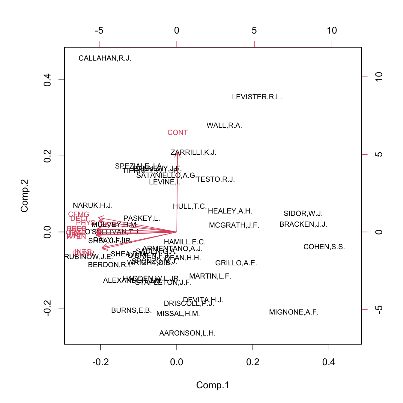 The \(\text{PC}_1\) gives a lawyer indicator of how badly the judge conducts a trial. The variable
 CONT, which measures the number of contacts between judge and lawyer, is almost uncorrelated with the rest of variables and is captured by \(\text{PC}_2\) (hence the rates of the lawyers are not affected by the number of contacts with the judge). We can identify the high-rated and low-rated judges in the left and right of the plot, respectively.
Let’s see an application of the biplot in La Liga 2015/2016, a dataset with more variables and a harder interpretation of PCs.
# Weights and biplot
pcaLaliga$loadings
##
## Loadings:
## Comp.1 Comp.2 Comp.3 Comp.4 Comp.5 Comp.6 Comp.7
## Points 0.280 0.136 0.145 0.137
## Wins 0.277 0.219 0.146
## Draws -0.157 -0.633 0.278 0.332 -0.102 0.382
## Loses -0.269 -0.118 -0.215 -0.137 -0.131 -0.313
## Goals.scored 0.271 -0.220 -0.101
## Goals.conceded -0.232 -0.336 -0.178 0.374
## Difference.goals 0.288 -0.171
## Percentage.scored.goals 0.271 -0.219
## Percentage.conceded.goals -0.232 -0.336 -0.178 0.375
## Shots 0.229 -0.299 -0.133 -0.325 -0.272 0.249
## Shots.on.goal 0.252 -0.265 -0.209
## Penalties.scored 0.160 -0.272 -0.410 0.636 -0.389 -0.160
## Assistances 0.271 -0.186 -0.158 0.129 0.176
## Fouls.made -0.189 0.561 0.178 0.213 0.592
## Matches.without.conceding 0.222 0.364 0.163 0.138 0.105 -0.239
## Yellow.cards -0.244 -0.108 0.358 -0.161 0.144
## Red.cards -0.158 -0.340 0.594 -0.192 -0.385 -0.303
## Offsides 0.163 -0.341 0.453 0.426 0.429 -0.283
## Comp.8 Comp.9 Comp.10 Comp.11 Comp.12 Comp.13 Comp.14
## Points 0.135 0.290 0.137 0.213
## Wins 0.263 0.120 0.230
## Draws 0.150 0.126 -0.249
## Loses -0.220 -0.338 -0.171 -0.103 -0.154
## Goals.scored -0.129 0.104 -0.251 0.238 0.289 -0.225 -0.260
## Goals.conceded 0.103 0.225 0.144 0.424
## Difference.goals -0.125 -0.272 0.151 -0.109 -0.374
## Percentage.scored.goals -0.132 0.103 -0.251 0.252 0.297 -0.223 0.501
## Percentage.conceded.goals 0.231 0.161 -0.601
## Shots 0.236 -0.267 0.452 -0.478 0.188
## Shots.on.goal -0.471 0.325 -0.439 0.488 0.192
## Penalties.scored 0.131 0.328
## Assistances 0.154 -0.570 -0.458 -0.504
## Fouls.made -0.363 -0.187 0.135 0.108 -0.135
## Matches.without.conceding 0.282 -0.303 0.388 0.258 -0.554
## Yellow.cards 0.733 -0.369 -0.152 0.219
## Red.cards 0.384 0.216 -0.127
## Offsides -0.302 -0.255 -0.146 0.128
## Comp.15 Comp.16 Comp.17 Comp.18
## Points 0.720 0.401
## Wins -0.272 0.741 -0.267
## Draws 0.118 0.337
## Loses 0.401 0.566 0.136
## Goals.scored 0.511 0.244 -0.438
## Goals.conceded 0.477 -0.181 0.324
## Difference.goals 0.103 -0.375 0.104 0.672
## Percentage.scored.goals -0.568
## Percentage.conceded.goals -0.422
## Shots
## Shots.on.goal
## Penalties.scored
## Assistances
## Fouls.made
## Matches.without.conceding
## Yellow.cards
## Red.cards
## Offsides
##
## Comp.1 Comp.2 Comp.3 Comp.4 Comp.5 Comp.6 Comp.7 Comp.8 Comp.9
## SS loadings 1.000 1.000 1.000 1.000 1.000 1.000 1.000 1.000 1.000
## Proportion Var 0.056 0.056 0.056 0.056 0.056 0.056 0.056 0.056 0.056
## Cumulative Var 0.056 0.111 0.167 0.222 0.278 0.333 0.389 0.444 0.500
## Comp.10 Comp.11 Comp.12 Comp.13 Comp.14 Comp.15 Comp.16 Comp.17
## SS loadings 1.000 1.000 1.000 1.000 1.000 1.000 1.000 1.000
## Proportion Var 0.056 0.056 0.056 0.056 0.056 0.056 0.056 0.056
## Cumulative Var 0.556 0.611 0.667 0.722 0.778 0.833 0.889 0.944
## Comp.18
## SS loadings 1.000
## Proportion Var 0.056
## Cumulative Var 1.000biplot(pcaLaliga, cex = 0.75)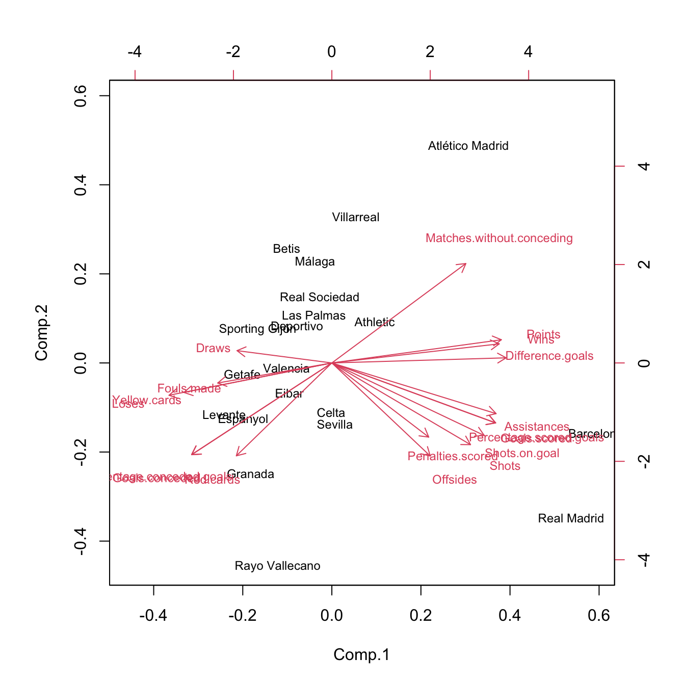 Some interesting highlights:
- \(\text{PC}_1\) can be regarded as the non-performance of a team during the season. It is negatively correlated with
Wins,Points,… and positively correlated withDraws,Loses,Yellow.cards,… The best performing teams are not surprising: Barcelona, Real Madrid and Atlético Madrid. On the other hand, among the worst-performing teams are Levante, Getafe and Granada. - \(\text{PC}_2\) can be seen as the inefficiency of a team (conceding points with little participation in the game). Using this interpretation we can see that Rayo Vallecano and Real Madrid were the most inefficient teams and Atlético Madrid and Villareal were the most efficient.
Offsidesis approximately uncorrelated withRed.cards.- \(\text{PC}_3\) does not have a clear interpretation.
If you are wondering about the 3D representation of the biplot, it can be computed through:
# Install this package with install.packages("pca3d")
library(pca3d)
pca3d(pcaLaliga, show.labels = TRUE, biplot = TRUE)
Finally, we mention that R Commander has a menu entry for performing PCA: 'Statistics' -> 'Dimensional analysis' -> 'Principal-components analysis...'. Alternatively, the plug-in FactoMineR implements a PCA with more options and graphical outputs. It can be loaded (if installed) in 'Tools' -> 'Load Rcmdr plug-in(s)...' -> 'RcmdPlugin.FactoMineR' (you will need to restart R Commander). For performing a PCA in FactoMineR, go to 'FactoMineR' -> 'Principal Component Analysis (PCA)'. In that menu you will have more advanced options than in R Commander’s PCA.