2.7 ANOVA and model fit

2.7.1 ANOVA

As we have seen in Sections 2.5 and 2.6, the variance of the error, $\sigma^2$, plays a fundamental role in the inference for the model coefficients and prediction. In this section we will see how the variance of $Y$ is decomposed into two parts, each one corresponding to the regression and to the error, respectively. This decomposition is called the ANalysis Of VAriance (ANOVA).

Before explaining ANOVA, it is important to recall an interesting result: the mean of the fitted values $\hat Y_1,\ldots,\hat Y_n$ is the mean of $Y_1,\ldots, Y_n$. This is easily seen if we plug-in the expression of $\hat\beta_0$: $$\begin{align*} \frac{1}{n}\sum_{i=1}^n \hat Y_i=\frac{1}{n}\sum_{i=1}^n \left(\hat \beta_0+\hat\beta_1X_i\right)=\hat \beta_0+\hat\beta_1\bar X=\left(\bar Y - \hat\beta_1\bar X \right) + \hat\beta_1\bar X=\bar Y. \end{align*}$$ The ANOVA decomposition considers the following measures of variation related with the response:

• $\text{SST}=\sum_{i=1}^n\left(Y_i-\bar Y\right)^2$, the total sum of squares. This is the total variation of $Y_1,\ldots,Y_n$, since $\text{SST}=ns_y^2$, where $s_y^2$ is the sample variance of $Y_1,\ldots,Y_n$.
• $\text{SSR}=\sum_{i=1}^n\left(\hat Y_i-\bar Y\right)^2$, the regression sum of squares¹². This is the variation explained by the regression line, that is, the variation from $\bar Y$ that is explained by the estimated conditional mean $\hat Y_i=\hat\beta_0+\hat\beta_1X_i$. $\text{SSR}=ns_{\hat y}^2$, where $s_{\hat y}^2$ is the sample variance of $\hat Y_1,\ldots,\hat Y_n$.
• $\text{SSE}=\sum_{i=1}^n\left(Y_i-\hat Y_i\right)^2$, the sum of squared errors¹³. Is the variation around the conditional mean. Recall that $\text{SSE}=\sum_{i=1}^n \hat\varepsilon_i^2=(n-2)\hat\sigma^2$, where $\hat\sigma^2$ is the sample variance of $\hat \varepsilon_1,\ldots,\hat \varepsilon_n$.

The ANOVA decomposition is $$\begin{align} \underbrace{\text{SST}}_{\text{Variation of }Y_i's} = \underbrace{\text{SSR}}_{\text{Variation of }\hat Y_i's} + \underbrace{\text{SSE}}_{\text{Variation of }\hat \varepsilon_i's} \tag{2.11} \end{align}$$ or, equivalently (dividing by $n$ in (2.11)), $$\begin{align*} \underbrace{s_y^2}_{\text{Variance of }Y_i's} = \underbrace{s_{\hat y}^2}_{\text{Variance of }\hat Y_i's} + \underbrace{(n-2)/n\times\hat\sigma^2}_{\text{Variance of }\hat\varepsilon_i's}. \end{align*}$$ The graphical interpretation of (2.11) is shown in Figures 2.24 and 2.25.

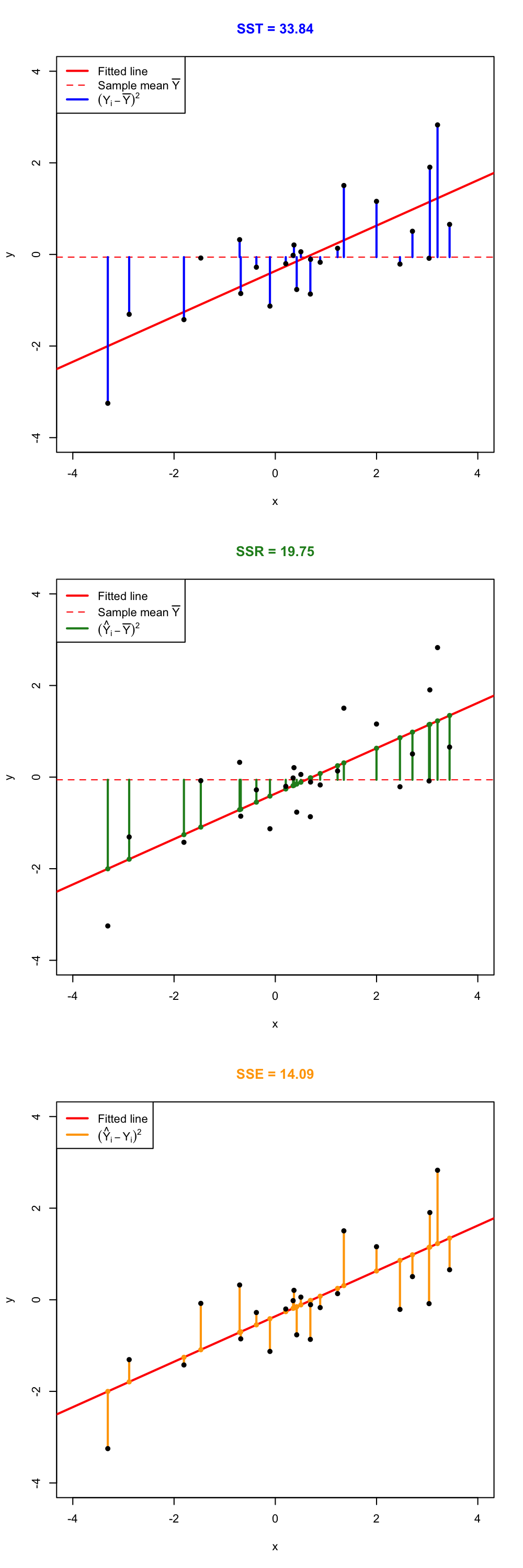
Figure 2.24: Visualization of the ANOVA decomposition. SST measures the variation of $Y_1,\ldots,Y_n$ with respect to $\bar Y$. SST measures the variation with respect to the conditional means, $\hat \beta_0+\hat\beta_1X_i$. SSE collects the variation of the residuals.

Figure 2.25: Illustration of the ANOVA decomposition and its dependence on $\sigma^2$ and $\hat\sigma^2$. Application also available here.

The ANOVA table summarizes the decomposition of the variance. Here is given in the layout employed by R.

	Degrees of freedom	Sum Squares	Mean Squares	$F$-value	$p$-value
Predictor	$1$	SSR	$\frac{\text{SSR}}{1}$	$\frac{\text{SSR}/1}{\text{SSE}/(n-2)}$	$p$
Residuals	$n - 2$	SSE	$\frac{\text{SSE}}{n-2}$

The anova function in R takes a model as an input and returns the ANOVA table. In R Commander, the ANOVA table can be computed by going to 'Models' -> 'Hypothesis tests' -> 'ANOVA table...'. In the 'Type of Tests' option, select 'Sequential ("Type I")'. (This types anova() for you…)

# Fit a linear model (alternatively, using R Commander)
model <- lm(MathMean ~ ReadingMean, data = pisa)
summary(model)
## 
## Call:
## lm(formula = MathMean ~ ReadingMean, data = pisa)
## 
## Residuals:
##     Min      1Q  Median      3Q     Max 
## -29.039 -10.151  -2.187   7.804  50.241 
## 
## Coefficients:
##              Estimate Std. Error t value Pr(>|t|)    
## (Intercept) -62.65638   19.87265  -3.153  0.00248 ** 
## ReadingMean   1.13083    0.04172  27.102  < 2e-16 ***
## ---
## Signif. codes:  0 '***' 0.001 '**' 0.01 '*' 0.05 '.' 0.1 ' ' 1
## 
## Residual standard error: 15.72 on 63 degrees of freedom
## Multiple R-squared:  0.921,  Adjusted R-squared:  0.9198 
## F-statistic: 734.5 on 1 and 63 DF,  p-value: < 2.2e-16

# ANOVA table
anova(model)
## Analysis of Variance Table
## 
## Response: MathMean
##             Df Sum Sq Mean Sq F value    Pr(>F)    
## ReadingMean  1 181525  181525  734.53 < 2.2e-16 ***
## Residuals   63  15569     247                      
## ---
## Signif. codes:  0 '***' 0.001 '**' 0.01 '*' 0.05 '.' 0.1 ' ' 1

The “$F$-value” of the ANOVA table represents the value of the $F$-statistic $\frac{\text{SSR}/1}{\text{SSE}/(n-2)}$. This statistic is employed to test $$\begin{align*} H_0:\beta_1=0\quad\text{vs.}\quad H_1:\beta_1\neq 0, \end{align*}$$ that is, the hypothesis of no linear dependence of $Y$ on $X$. The result of this test is completely equivalent to the $t$-test for $\beta_1$ that we saw in Section 2.5 (this is something specific for simple linear regression – the $F$-test will not be equivalent to the $t$-test for $\beta_1$ in Chapter 3). It happens that $$\begin{align*} F=\frac{\text{SSR}/1}{\text{SSE}/(n-2)}\stackrel{H_0}{\sim} F_{1,n-2}, \end{align*}$$ where $F_{1,n-2}$ is the Snedecor’s $F$ distribution¹⁴ with $1$ and $n-2$ degrees of freedom. If $H_0$ is true, then $F$ is expected to be small since SSR will be close to zero. The $p$-value of this test is the same as the $p$-value of the $t$-test for $H_0:\beta_1=0$.

Recall that the $F$-statistic, its $p$-value and the degrees of freedom are also given in the output of summary.

For the y6 ~ x6 and y7 ~ x7 in the assumptions dataset, compute their ANOVA tables. Check that the $p$-values of the $t$-test for $\beta_1$ and the $F$-test are the same.

2.7.2 The $R^2$

The coefficient of determination $R^2$ is closely related with the ANOVA decomposition. $R^2$ is defined as $$\begin{align*} R^2=\frac{\text{SSR}}{\text{SST}}=\frac{\text{SSR}}{\text{SSR}+\text{SSE}}=\frac{\text{SSR}}{\text{SSR}+(n-2)\hat\sigma^2}. \end{align*}$$ $R^2$ measures the proportion of variation of the response variable $Y$ that is explained by the predictor $X$ through the regression. The proportion of total variation of $Y$ that is not explained is $1-R^2=\frac{\text{SSE}}{\text{SST}}$. Intuitively, $R^2$ measures the tightness of the data cloud around the regression line, since is related directly with $\hat\sigma^2$. Check in Figure 2.25 how changing the value of $\sigma^2$ (not $\hat\sigma^2$, but $\hat\sigma^2$ is obviously dependent on $\sigma^2$) affects the $R^2$.

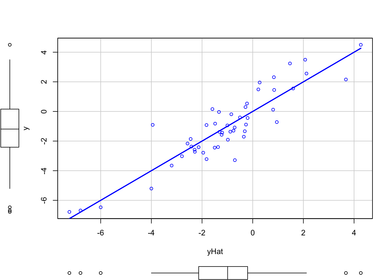
The $R^2$ is related with the sample correlation coefficient $$\begin{align*} r_{xy}=\frac{s_{xy}}{s_xs_y}=\frac{\sum_{i=1}^n \left(X_i-\bar X \right)\left(Y_i-\bar Y \right)}{\sqrt{\sum_{i=1}^n \left(X_i-\bar X \right)^2}\sqrt{\sum_{i=1}^n \left(Y_i-\bar Y \right)^2}} \end{align*}$$ and it can be seen that $R^2=r_{xy}^2$. Interestingly, it also holds that $R^2=r^2_{y\hat y}$, that is, the square of the sample correlation coefficient between $Y_1,\ldots,Y_n$ and $\hat Y_1,\ldots,\hat Y_n$ is $R^2$, a fact that is not immediately evident. This can be easily by first noting that $$\begin{align} \hat Y_i=\hat\beta_0+\hat\beta_1X_i=(\bar Y-\hat\beta_1X_i)+\hat\beta_1X_i=\bar Y+\hat\beta_1(X_i-\bar X) \tag{2.12} \end{align}$$ and then replacing (2.12) into $$\begin{align*} r^2_{y\hat y}=\frac{s_{y\hat y}^2}{s_y^2s_{\hat y}^2}=\frac{\left(\sum_{i=1}^n \left(Y_i-\bar Y \right)\left(\hat Y_i-\bar Y \right)\right)^2}{\sum_{i=1}^n \left(Y_i-\bar Y \right)^2\sum_{i=1}^n \left(\hat Y_i-\bar Y \right)^2}=\frac{\left(\sum_{i=1}^n \left(Y_i-\bar Y \right)\left(\bar Y+\hat\beta_1(X_i-\bar X)-\bar Y \right)\right)^2}{\sum_{i=1}^n \left(Y_i-\bar Y \right)^2\sum_{i=1}^n \left(\bar Y+\hat\beta_1(X_i-\bar X)-\bar Y \right)^2}=r^2_{xy}. \end{align*}$$

The equality $R^2=r^2_{y \hat y}$ is still true for the multiple linear regression, e.g. $Y=\beta_0+\beta_1X_1+\beta_2X_2+\varepsilon$. On the contrary, there is no coefficient of correlation between three or more variables, so $r_{x_1x_2y}$ does not exist. Hence, $R^2=r^2_{x y}$ is a specific fact for simple linear regression.

The result $R^2=r^2_{xy}=r^2_{y\hat y}$ can be checked numerically and graphically with the next code.

# Responses generated following a linear model
set.seed(343567) # Fixes seed, allows to generate the same random data
x <- rnorm(50)
eps <- rnorm(50)
y <- -1 + 2 * x + eps

# Regression model
reg <- lm(y ~ x)
yHat <- reg$fitted.values

# Summary
summary(reg)
## 
## Call:
## lm(formula = y ~ x)
## 
## Residuals:
##     Min      1Q  Median      3Q     Max 
## -2.5834 -0.6015 -0.1466  0.6006  3.0419 
## 
## Coefficients:
##             Estimate Std. Error t value Pr(>|t|)    
## (Intercept)  -0.9027     0.1503  -6.007 2.45e-07 ***
## x             2.1107     0.1443  14.623  < 2e-16 ***
## ---
## Signif. codes:  0 '***' 0.001 '**' 0.01 '*' 0.05 '.' 0.1 ' ' 1
## 
## Residual standard error: 1.059 on 48 degrees of freedom
## Multiple R-squared:  0.8167, Adjusted R-squared:  0.8129 
## F-statistic: 213.8 on 1 and 48 DF,  p-value: < 2.2e-16

# Square of the correlation coefficient
cor(y, x)^2
## [1] 0.8166752
cor(y, yHat)^2
## [1] 0.8166752

# Plots
scatterplot(y ~ x, smooth = FALSE)
scatterplot(y ~ yHat, smooth = FALSE)

We conclude this section by pointing out two common sins regarding the use of $R^2$. First, recall two important concepts regarding the application of any regression model in practice, in particular the linear model:

1. Correctness. The linear model is built on certain assumptions, such as the ones we saw in Section 2.4. All the inferential results are based on these assumptions being true!¹⁵. A model is formally correct whenever the assumptions on which is based are not violated in the data.

2. Usefulness. The usefulness of the model is a more subjective concept, but is usually measured by the accuracy on the prediction and explanation of the response $Y$ by the predictor $X$. For example, $Y=0X+\varepsilon$ is a valid linear model, but is completely useless for predicting $Y$ from $X$.

Figure 2.25 show a fitted regression line to a small dataset, for various levels of $\sigma^2$. All the linear models are correct by construction, but the ones with a larger $R^2$ are more useful for predicting/explaining $Y$ from $X$, since this is done in a more precise way.

$R^2$ does not measure the correctness of a linear model but its usefulness (for prediction, for explaining the variance of $Y$), assuming the model is correct.

Trusting blindly the $R^2$ can lead to catastrophic conclusions, since the model may not be correct. Here is a counterexample of a linear regression performed in a data that clearly does not satisfy the assumptions discussed in Section 2.4, but despite so it has a large $R^2$. Recall how biased will be the predictions for $x=0.35$ and $x=0.65$!

# Create data that:
# 1) does not follow a linear model
# 2) the error is heteroskedastic
x <- seq(0.15, 1, l = 100)
set.seed(123456)
eps <- rnorm(n = 100, sd = 0.25 * x^2)
y <- 1 - 2 * x * (1 + 0.25 * sin(4 * pi * x)) + eps

# Great R^2!?
reg <- lm(y ~ x)
summary(reg)
## 
## Call:
## lm(formula = y ~ x)
## 
## Residuals:
##      Min       1Q   Median       3Q      Max 
## -0.53525 -0.18020  0.02811  0.16882  0.46896 
## 
## Coefficients:
##             Estimate Std. Error t value Pr(>|t|)    
## (Intercept)  0.87190    0.05860   14.88   <2e-16 ***
## x           -1.69268    0.09359  -18.09   <2e-16 ***
## ---
## Signif. codes:  0 '***' 0.001 '**' 0.01 '*' 0.05 '.' 0.1 ' ' 1
## 
## Residual standard error: 0.232 on 98 degrees of freedom
## Multiple R-squared:  0.7695, Adjusted R-squared:  0.7671 
## F-statistic: 327.1 on 1 and 98 DF,  p-value: < 2.2e-16

# But prediction is obviously problematic
scatterplot(y ~ x, smooth = FALSE)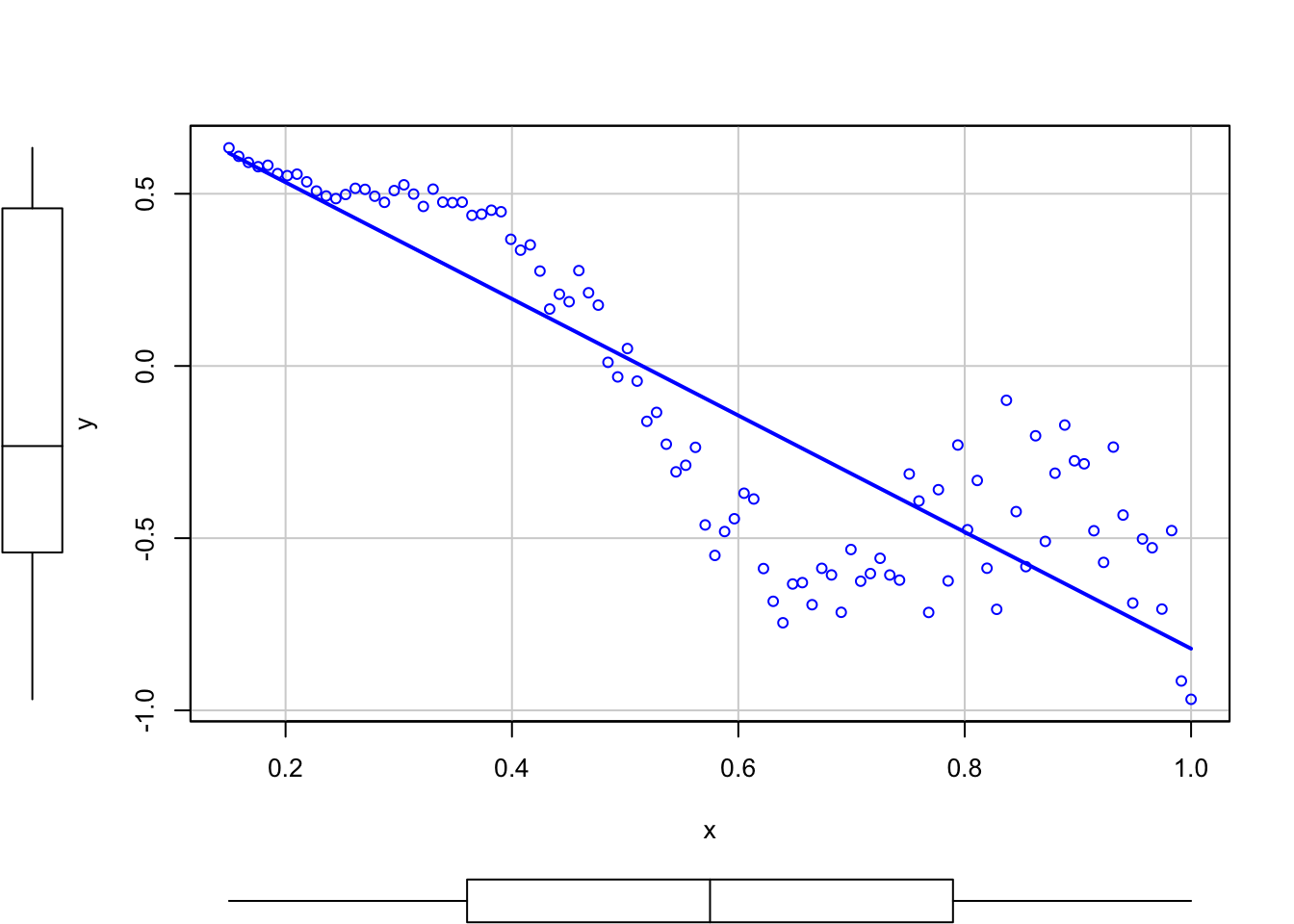

So remember:

A large $R^2$ means nothing if the assumptions of the model do not hold. $R^2$ is the proportion of variance of $Y$ explained by $X$, but, of course, only when the linear model is correct.

---

12. Recall that SSR is different from RSS (Residual Sum of Squares, Section 2.3).↩︎

13. Recall that SSE and RSS (for $(\hat \beta_0,\hat \beta_1)$) are just different names for referring to the same quantity: $\text{SSE}=\sum_{i=1}^n\left(Y_i-\hat Y_i\right)^2=\sum_{i=1}^n\left(Y_i-\hat \beta_0-\hat \beta_1X_i\right)^2=\mathrm{RSS}\left(\hat \beta_0,\hat \beta_1\right)$.↩︎

14. The $F_{n,m}$ distribution arises as the quotient of two independent random variables $\chi^2_n$ and $\chi^2_m$, $\frac{\chi^2_n/n}{\chi^2_m/m}$.↩︎

15. If the assumptions are not satisfied (mismatch between what is assumed to happen in theory and what the data is), then the inference results may be misleading.↩︎