2.8 Nonlinear relationships
The linear model is termed linear not because the regression curve is a line, but because the effects of the parameters \(\beta_0\) and \(\beta_1\) are linear. Indeed, the predictor \(X\) may exhibit a nonlinear effect on the response \(Y\) and still be a linear model! For example, the following models can be transformed into simple linear models:
- \(Y=\beta_0+\beta_1X^2+\varepsilon\)
- \(Y=\beta_0+\beta_1\log(X)+\varepsilon\)
- \(Y=\beta_0+\beta_1(X^3-\log(|X|) + 2^X)+\varepsilon\)
The trick is to work with the transformed predictor (\(X^2\), \(\log(X)\), …), instead of with the original variable \(X\). Then, rather than working with the sample \((X_1,Y_1),\ldots,(X_n,Y_n)\), we consider the transformed sample \((\tilde X_1,Y_1),\ldots,(\tilde X_n,Y_n)\) with (for the above examples):
- \(\tilde X_i=X_i^2\), \(i=1,\ldots,n\).
- \(\tilde X_i=\log(X_i)\), \(i=1,\ldots,n\).
- \(\tilde X_i=X_i^3-\log(|X_i|) + 2^{X_i}\), \(i=1,\ldots,n\).
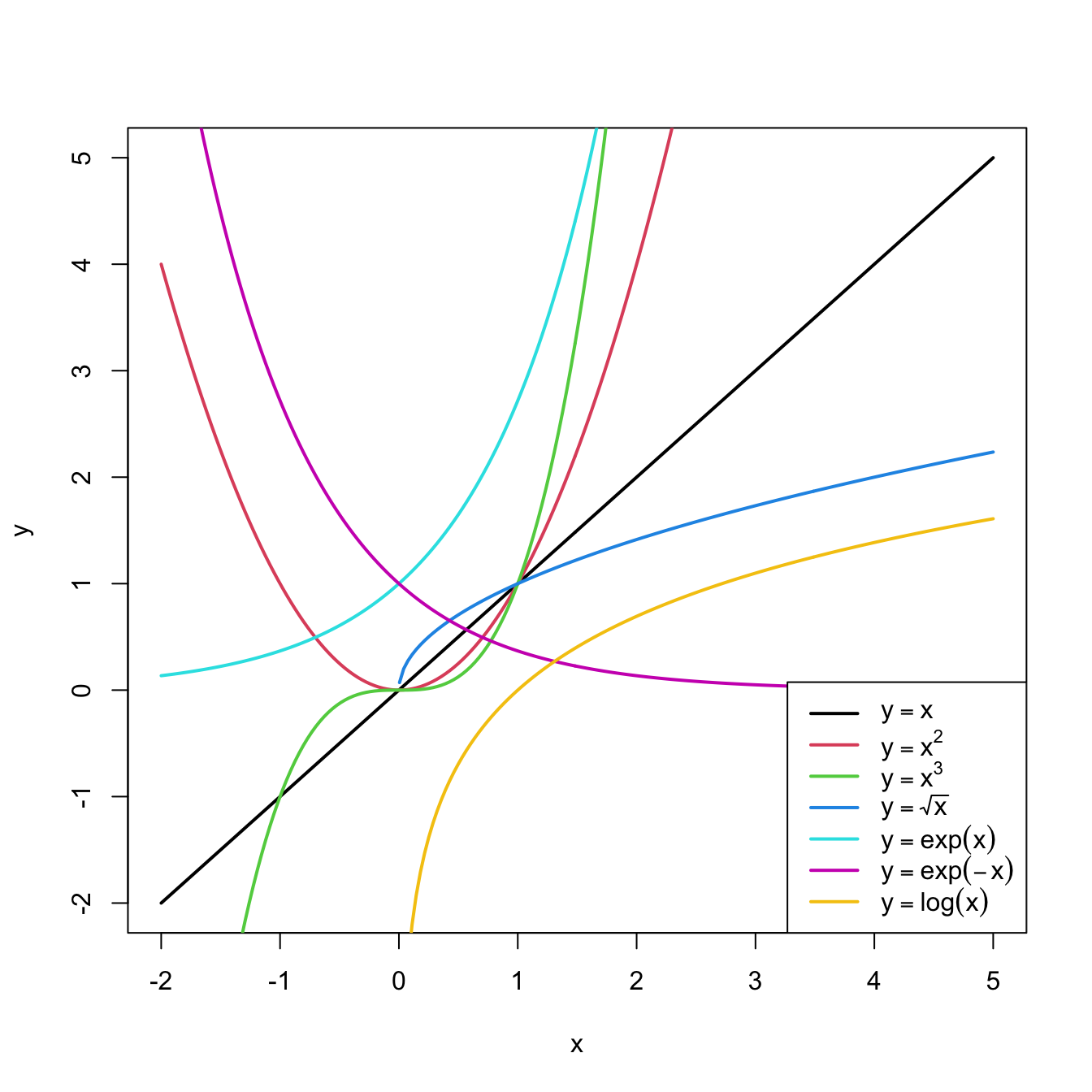
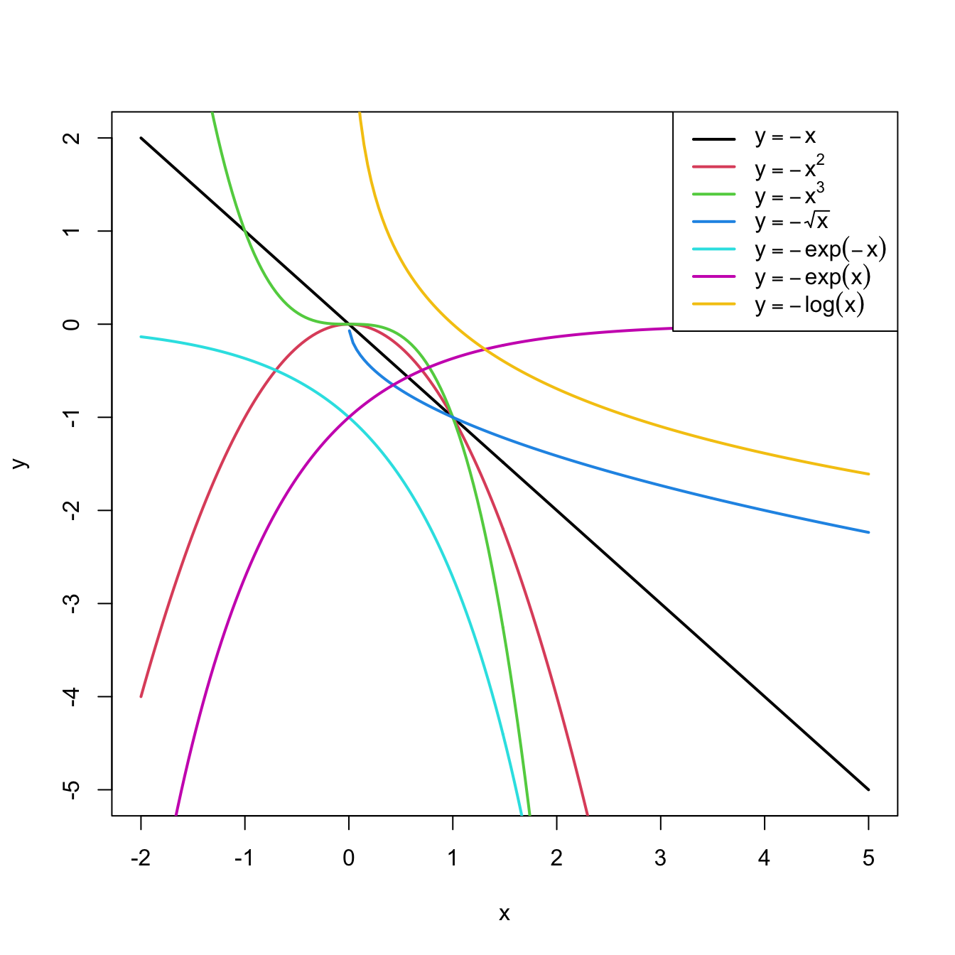
Figure 2.26: Some common nonlinear transformations and their negative counterparts. Recall the domain of definition of each transformation.
An example of this simple but powerful trick is given as follows. The left panel of Figure 2.27 shows the scatterplot for some data y and x, together with its fitted regression line. Clearly, the data does not follow a linear pattern, but a nonlinear one. In order to identify which one might be, we compare it against the set of mathematical functions displayed in Figure 2.26. We see that the shape of the point cloud is similar to \(y=x^2\). Hence, y might be better explained by the square of x, x^2, rather than by x. Indeed, if we plot y against x^2 in the right panel of Figure 2.27, we can see that the fit of the regression line is much better.
In conclusion, with a simple trick we have increased drastically the explanation of the response. However, there is a catch: knowing which transformation is required in order to linearise the relation between response and the predictor is a kind of art which requires some good eye. This is partially alleviated by the extension of this technique to deal with polynomials rather than monomials, as we will see in Chapter 3. For the moment, we will consider only the transformations displayed in Figure 2.26. Figure 2.28 shows different transformations linearizing nonlinear data patterns.
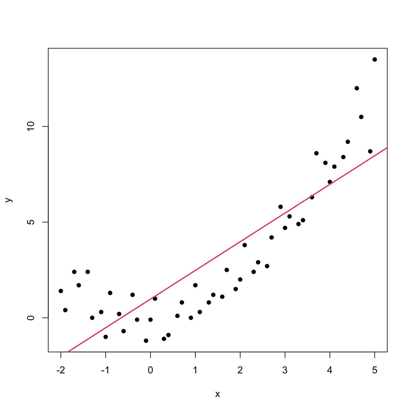
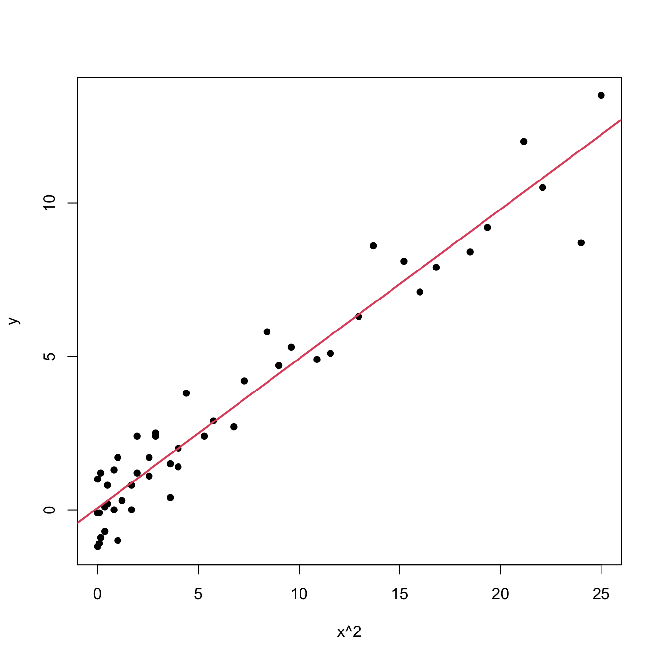
Figure 2.27: Left: quadratic pattern when plotting \(Y\) against \(X\). Right: linearized pattern when plotting \(Y\) against \(X^2\).
If you apply a nonlinear transformation, namely \(f\), and fit the linear model \(Y=\beta_0+\beta_1 f(X)+\varepsilon\), then there is no point in fit also the model resulting from the negative transformation \(-f\). The model with \(-f\) is exactly the same as the one with \(f\) but with the sign of \(\beta_1\) flipped!
As a rule of thumb, use Figure 2.26 with the transformations to compare it with the data pattern, then choose the most similar curve and finally apply the corresponding function with positive sign.Figure 2.28: Illustration of the choice of the nonlinear transformation. Application also available here.
logGDPp instead of GDPp due to its higher linearity with MathMean).
Let’s see how we can compute transformations of our predictors and perform a linear regression with them. The data for the above example is the following:
# Data
x <- c(-2, -1.9, -1.7, -1.6, -1.4, -1.3, -1.1, -1, -0.9, -0.7, -0.6,
       -0.4, -0.3, -0.1, 0, 0.1, 0.3, 0.4, 0.6, 0.7, 0.9, 1, 1.1, 1.3,
       1.4, 1.6, 1.7, 1.9, 2, 2.1, 2.3, 2.4, 2.6, 2.7, 2.9, 3, 3.1,
       3.3, 3.4, 3.6, 3.7, 3.9, 4, 4.1, 4.3, 4.4, 4.6, 4.7, 4.9, 5)
y <- c(1.4, 0.4, 2.4, 1.7, 2.4, 0, 0.3, -1, 1.3, 0.2, -0.7, 1.2, -0.1,
       -1.2, -0.1, 1, -1.1, -0.9, 0.1, 0.8, 0, 1.7, 0.3, 0.8, 1.2, 1.1,
       2.5, 1.5, 2, 3.8, 2.4, 2.9, 2.7, 4.2, 5.8, 4.7, 5.3, 4.9, 5.1,
       6.3, 8.6, 8.1, 7.1, 7.9, 8.4, 9.2, 12, 10.5, 8.7, 13.5)

# Data frame (a matrix with column names)
nonLinear <- data.frame(x = x, y = y)
In order to perform a simple linear regression in x^2, and not in x, we need to compute a new variable in our dataset that contains the square of x. We can do it in two equivalent ways:
Through R Commander. In Section 2.1.2 we saw how to create a new variable in our active dataset (remember Figure 2.8). Go to
'Data' -> 'Manage variables in active dataset...' -> 'Compute new variable...'. Set the'New variable name'tox2and the'Expression to compute'tox^2.Through R. Just type:
# We create a new column inside nonLinear, called x2, that contains
# nonLinear$x^2
nonLinear$x2 <- nonLinear$x^2

# Check the variables
names(nonLinear)
## [1] "x"  "y"  "x2"
With either the two previous points you will have a new variable called x2. If you wish to remove it, you can do it by either typing
# Empties the column named x2
nonLinear$x2 <- NULL
or, in R Commander, by going to 'Data' -> 'Manage variables in active data set' -> 'Delete variables from data set...' and select to remove x2.
Now we are ready to perform the regression. If you do it directly through R, you will obtain:
mod1 <- lm(y ~ x, data = nonLinear)
summary(mod1)
##
## Call:
## lm(formula = y ~ x, data = nonLinear)
##
## Residuals:
##     Min      1Q  Median      3Q     Max
## -2.5268 -1.7513 -0.4017  0.9750  5.0265
##
## Coefficients:
##             Estimate Std. Error t value Pr(>|t|)
## (Intercept)   0.9771     0.3506   2.787   0.0076 **
## x             1.4993     0.1374  10.911 1.35e-14 ***
## ---
## Signif. codes:  0 '***' 0.001 '**' 0.01 '*' 0.05 '.' 0.1 ' ' 1
##
## Residual standard error: 2.005 on 48 degrees of freedom
## Multiple R-squared:  0.7126, Adjusted R-squared:  0.7067
## F-statistic:   119 on 1 and 48 DF,  p-value: 1.353e-14
mod2 <- lm(y ~ x2, data = nonLinear)
summary(mod2)
##
## Call:
## lm(formula = y ~ x2, data = nonLinear)
##
## Residuals:
##     Min      1Q  Median      3Q     Max
## -3.0418 -0.5523 -0.1465  0.6286  1.8797
##
## Coefficients:
##             Estimate Std. Error t value Pr(>|t|)
## (Intercept)  0.05891    0.18462   0.319    0.751
## x2           0.48659    0.01891  25.725   <2e-16 ***
## ---
## Signif. codes:  0 '***' 0.001 '**' 0.01 '*' 0.05 '.' 0.1 ' ' 1
##
## Residual standard error: 0.9728 on 48 degrees of freedom
## Multiple R-squared:  0.9324, Adjusted R-squared:  0.931
## F-statistic: 661.8 on 1 and 48 DF,  p-value: < 2.2e-16
A fast way of performing and summarizing the quadratic fit is
summary(lm(y ~ I(x^2), data = nonLinear))Some remarks about this expression:
-
The
I()function wrappingx^2is fundamental when applying arithmetic operations in the predictor. The symbols+,*,^, … have different meaning when imputed in a formula, so is required to useI()to indicate that they must be interpreted in their arithmetic meaning and that the result of the expression denotes a new predictor variable. For example, useI((x - 1)^3 - log(3 * x))if you want to apply the transformation(x - 1)^3 - log(3 * x). -
We are computing the
summaryoflmdirectly, without using an intermediate variable for storing the output oflm. This is perfectly valid and very handy, but note that you will not be able to access the information outputted bylm, only the one fromsummary.
Load the dataset assumptions.RData. We are going to work with the regressions y2 ~ x2, y3 ~ x3, y8 ~ x8 and y9 ~ x9, in order to identify which transformation of Figure 2.26 gives the best fit. (For the purpose of illustration, we do not care if the assumptions are respected.) For these, do the following:
- Find the transformation that yields the largest \(R^2\).
- Compare the original and the transformed linear models.
Some hints:
y2 ~ x2has a negative dependence, so look at the right panel of the transformations figure.y3 ~ x3seems to have just a subtle nonlinearity… Will it be worth to attempt a transformation?- For
y9 ~ x9, try with also withexp(-abs(x9)),log(abs(x9))and2^abs(x9). (abscomputes the absolute value.)