Chapter 4 Matrix Models I: Intro to MPMs, and Raw (Empirical) MPMs
An ounce of algebra is worth a ton of verbal argument.
Note: The example code in this chapter relies on code executed in previous chapters. This code is available in a ready-to-run block in Appendix II (19.0.2).
Matrix projection models (MPMs) are representations of the dynamics of a population across all life history stages deemed relevant, across the most relevant time interval (typically one year, but sometimes different, and assumed to be consistent within each analysis). In the simplest MPMs, matrix elements (\(a_{kj}\)) show either the probability of transition for an individual in stage \(j\) at occasion t (along the columns), to stage \(k\) at occasion t+1 (along the rows), or the mean rate of production of offspring into stage \(k\) at occasion t+1 (along the rows) by adult individuals in reproductive stage \(j\) in occasion t (along the columns). Conceptually, each individual is in a particular stage in the instance of monitoring or observation, and then either dies or completes a transition in the interval between that observation occasion and the next. Death is not an explicit life stage and so is not modeled as such, instead becoming a potential endpoint of each transition.
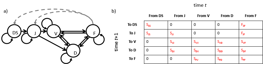
Figure 4.1 shows a simple matrix that assumes five stages in the Cypripedium candidum life cycle. These stages are dormant seed (S), juvenile (J, comprised of protocorms and seedlings), non-flowering but sprouting adult (V), non-sprouting adult (D), and flowering adult (F). In equation (4.1), we project a column vector of numbers of individuals alive in each stage in time 1 (e.g., \(n _{1,S}\) is the number of individuals in stage \(S\) in time 1) a single time step forward using standard matrix multiplication with the projection matrix. The product is another column vector showing the predicted numbers of individuals alive in each stage in the next occasion (e.g., \(n _{2,S}\) is the number of individuals in stage \(S\) in time 2).
\[\begin{equation} \left[\begin{array} {rrrrr} n _{2,S} \\ n _{2,J} \\ n _{2,V} \\ n _{2,D} \\ n _{2,F} \\ \end{array}\right] = \left[\begin{array} {ccccc} S_{SS} & 0 & 0 & 0 & F _{SF} \\ S_{JS} & S_{JJ} & 0 & 0 & F _{JF} \\ 0 & S_{VJ} & S_{VV} & S_{VD} & S _{VF} \\ 0 & S_{DJ} & S_{DV} & S_{DD} & S _{DF} \\ 0 & 0 & S_{FV} & S_{FD} & S _{FF} \\ \end{array}\right] \left[\begin{array} {rrrrr} n _{1,S} \\ n _{1,J} \\ n _{1,V} \\ n _{1,D} \\ n _{1,F} \\ \end{array}\right] \tag{4.1} \end{equation}\]
The total population size in any occasion is the sum of the numbers of individuals in all stages in that occasion, or in other words the sum of the elements in the column vector (these may first be rounded down to the nearest integer, to prevent fractional individuals being included). The true discrete population growth rate (\(\lambda\)) is calculated as the ratio of the true total population size in occasion t+1 to the true total population size in occasion t. Naturally, projections are estimates, so the estimated population growth rate (\(\hat{\lambda}\)) can be calculated as either the ratio of projected population size in time t+1 to projected population size in time t, or as the dominant eigenvalue of the projection matrix. In the latter case, estimated \(\hat{\lambda}\) is actually the expected population growth rate assuming that the population is at stable stage equilibrium, and so may differ from the true \(\lambda\) depending on conditions.
How does one estimate the elements composing the matrix? Let’s start with a general matrix, as follows. We start with \(m\) life history stages, and the column vectors denote the number of individuals in each of \(m\) stages in times \(t\) and \(t+1\). Element \(a _{1, m}\) refers to the transition rate from stage \(m\) in time \(t\) to stage \(1\) in time \(t+1\).
\[\begin{equation} \left[\begin{array} {rrr} n _{t+1,1} \\ \vdots \\ n _{t+1,m} \\ \end{array}\right] = \left[\begin{array} {ccc} a _{1,1} & \dots & a _{1,m} \\ \vdots & \ddots & \vdots \\ a _{m,1} & \dots & a _{m,m} \\ \end{array}\right] \left[\begin{array} {rrr} n _{t,1} \\ \vdots \\ n _{t,m} \\ \end{array}\right] \tag{4.2} \end{equation}\]
First, we note that there are two primary kinds of elements - survival-transition elements, and fecundity elements. The former are probabilities denoting the chance of transitioning from one stage in time t to another in time t+1, and the latter are rates denoting the number of offspring produced per reproductive individual in time t that survive to time t+1 (this is the pre-breeding model as described in Chapter 2, while fecundity in the post-breeding case would equal the survival of the reproductive parent from time t to time t+1 multiplied by the number of offspring produced). In the raw MPM (also called the empirical MPM), which is the first and still most commonly developed MPM, survival-transition elements are estimated as follows.
\[\begin{equation} a _{kj} = \frac{n _{kj}}{\sum_{i=1}^{d} n _{ij}} \tag{4.3} \end{equation}\]
Here, we can refer to matrix elements as \(a_{kj}\), where the element represents the rate at which individuals transition to stage \(k\) in occasion t+1 after having been stage \(j\) in occasion t. Then, \(n _{kj}\) is the number of individuals making this transition, and \(d\) is the number of stages plus death in the life history model (\(d=m+1\), where \(m\) is the number of life history stages). The denominator represents the total number of individuals alive in stage \(j\) in time t regardless of whether they are alive or dead in time t+1. For example, if 100 individuals are alive in stage D in year 2010, and 20 of these are alive in stage D in year 2011, as are a further 40 in stage V and a further 25 in stage F, then the associated transition probabilities are 0.20, 0.40, and 0.25, respectively. The overall survival probability for stage D is the sum of these transitions, or 0.85, with 15% of individuals alive in 2010 dying by the time of the monitoring occasion in 2011.
Fecundity in the pre-breeding model can be estimated as follows.
\[\begin{equation} a _{kj} = s_{k} \frac{\sum_{i=1}^{n_{.j}} fec_{i}}{ n _{.j}} \tag{4.4} \end{equation}\]
Here, \(s_{k}\) is the survival of newborns to the first-year stage from time t to time t+1, \(fec_{i}\) is the actual fecundity of individual \(i\) in time t, \(n_{.j}\) is the number of reproductive adults in stage \(j\) at time t, and the right-hand term, \(\frac{\sum_{i=1}^{n_{.j}} fec_{i}}{ n _{.j}}\), is the average offspring production per reproductive adult.
4.1 Developing raw MPMs
In package lefko3, the primary function to create basic raw MPMs is rlefko2(). In the code below, we use this function to create a series of raw matrices for our Cypripedium candidum dataset. In our call to rlefko2(), we need to provide R at the very least with the dataset that it will use to estimate the matrix (data = cypraw_v1), the stageframe identifying and describing all stages in the life history model (stageframe = cypframe_raw), and the names of the variables coding for stage in times t+1 and t (stages = c("stage3", "stage2")). Our call also includes a statement that we wish to estimate matrices for all occasions possible (year = "all", which also requires the identification of the monitoring time variable, yearcol = "year2"). We will also specify that we wish matrices to be estimated for all three patches (patch = "all", which also requires the identification of the patch variable, patchcol = "patchid"). This function assumes default variable names for most of the status variables in hfv datasets. Since we are using size variables other than the defaults, we need to supply those names (size = c("size3added", "size2added")). Finally, we will supply our supplement table (supplement = cypsupp2_raw), and note the name of the variable coding for individual identity (indivcol = "individ").
cypmatrix2rp <- rlefko2(data = cypraw_v1, stageframe = cypframe_raw,
year = "all", patch = "all", stages = c("stage3", "stage2"),
size = c("size3added", "size2added"), supplement = cypsupp2_raw,
yearcol = "year2", patchcol = "patchid", indivcol = "individ")
cypmatrix2rp
> $A
> $A[[1]]
> [,1] [,2] [,3] [,4] [,5] [,6] [,7] [,8] [,9] [,10]
> [1,] 0.08 0.0 0.0 0.00 0.0000000 0 0.0000000 500.0 1666.6666667 0
> [2,] 0.10 0.0 0.0 0.00 0.0000000 0 0.0000000 500.0 1666.6666667 0
> [3,] 0.00 0.1 0.0 0.00 0.0000000 0 0.0000000 0.0 0.0000000 0
> [4,] 0.00 0.0 0.1 0.00 0.0000000 0 0.0000000 0.0 0.0000000 0
> [5,] 0.00 0.0 0.0 0.05 0.0500000 0 0.0000000 0.0 0.0000000 0
> [6,] 0.00 0.0 0.0 0.00 0.0000000 0 0.0000000 0.0 0.0000000 0
> [7,] 0.00 0.0 0.0 0.00 0.4454545 0 0.6363636 0.2 0.0000000 0
> [8,] 0.00 0.0 0.0 0.00 0.1909091 0 0.2727273 0.6 0.6666667 1
> [9,] 0.00 0.0 0.0 0.00 0.0000000 0 0.0000000 0.2 0.3333333 0
> [10,] 0.00 0.0 0.0 0.00 0.0000000 0 0.0000000 0.0 0.0000000 0
> [11,] 0.00 0.0 0.0 0.00 0.0000000 0 0.0000000 0.0 0.0000000 0
> [,11]
> [1,] 0
> [2,] 0
> [3,] 0
> [4,] 0
> [5,] 0
> [6,] 0
> [7,] 0
> [8,] 0
> [9,] 0
> [10,] 0
> [11,] 0
>
> $A[[2]]
> [,1] [,2] [,3] [,4] [,5] [,6] [,7] [,8] [,9] [,10] [,11]
> [1,] 0.08 0.0 0.0 0.00 0.0000 0 312.500 1111.1111111 1250 0 0
> [2,] 0.10 0.0 0.0 0.00 0.0000 0 312.500 1111.1111111 1250 0 0
> [3,] 0.00 0.1 0.0 0.00 0.0000 0 0.000 0.0000000 0 0 0
> [4,] 0.00 0.0 0.1 0.00 0.0000 0 0.000 0.0000000 0 0 0
> [5,] 0.00 0.0 0.0 0.05 0.0500 0 0.000 0.0000000 0 0 0
> [6,] 0.00 0.0 0.0 0.00 0.0875 0 0.125 0.0000000 0 0 0
> [7,] 0.00 0.0 0.0 0.00 0.5250 0 0.750 0.3333333 0 0 0
> [8,] 0.00 0.0 0.0 0.00 0.0000 0 0.000 0.4444444 0 0 0
> [9,] 0.00 0.0 0.0 0.00 0.0000 0 0.000 0.2222222 1 0 0
> [10,] 0.00 0.0 0.0 0.00 0.0000 0 0.000 0.0000000 0 0 0
> [11,] 0.00 0.0 0.0 0.00 0.0000 0 0.000 0.0000000 0 0 0
>
> $A[[3]]
> [,1] [,2] [,3] [,4] [,5] [,6] [,7] [,8] [,9] [,10] [,11]
> [1,] 0.08 0.0 0.0 0.00 0.0000000 0 0.0000000 0 0.00 0 0
> [2,] 0.10 0.0 0.0 0.00 0.0000000 0 0.0000000 0 0.00 0 0
> [3,] 0.00 0.1 0.0 0.00 0.0000000 0 0.0000000 0 0.00 0 0
> [4,] 0.00 0.0 0.1 0.00 0.0000000 0 0.0000000 0 0.00 0 0
> [5,] 0.00 0.0 0.0 0.05 0.0500000 0 0.0000000 0 0.00 0 0
> [6,] 0.00 0.0 0.0 0.00 0.0000000 0 0.0000000 0 0.00 0 0
> [7,] 0.00 0.0 0.0 0.00 0.4666667 0 0.6666667 0 0.00 0 0
> [8,] 0.00 0.0 0.0 0.00 0.2333333 1 0.3333333 1 0.25 0 0
> [9,] 0.00 0.0 0.0 0.00 0.0000000 0 0.0000000 0 0.75 0 0
> [10,] 0.00 0.0 0.0 0.00 0.0000000 0 0.0000000 0 0.00 0 0
> [11,] 0.00 0.0 0.0 0.00 0.0000000 0 0.0000000 0 0.00 0 0
>
> $A[[4]]
> [,1] [,2] [,3] [,4] [,5] [,6] [,7] [,8] [,9] [,10]
> [1,] 0.08 0.0 0.0 0.00 0.0000000 0 0.0000000 0.0000000 0.0000000 0
> [2,] 0.10 0.0 0.0 0.00 0.0000000 0 0.0000000 0.0000000 0.0000000 0
> [3,] 0.00 0.1 0.0 0.00 0.0000000 0 0.0000000 0.0000000 0.0000000 0
> [4,] 0.00 0.0 0.1 0.00 0.0000000 0 0.0000000 0.0000000 0.0000000 0
> [5,] 0.00 0.0 0.0 0.05 0.0500000 0 0.0000000 0.0000000 0.0000000 0
> [6,] 0.00 0.0 0.0 0.00 0.1166667 0 0.1666667 0.2222222 0.0000000 0
> [7,] 0.00 0.0 0.0 0.00 0.3500000 0 0.5000000 0.4444444 0.3333333 0
> [8,] 0.00 0.0 0.0 0.00 0.0000000 0 0.0000000 0.3333333 0.3333333 0
> [9,] 0.00 0.0 0.0 0.00 0.0000000 0 0.0000000 0.0000000 0.3333333 0
> [10,] 0.00 0.0 0.0 0.00 0.0000000 0 0.0000000 0.0000000 0.0000000 0
> [11,] 0.00 0.0 0.0 0.00 0.0000000 0 0.0000000 0.0000000 0.0000000 0
> [,11]
> [1,] 0
> [2,] 0
> [3,] 0
> [4,] 0
> [5,] 0
> [6,] 0
> [7,] 0
> [8,] 0
> [9,] 0
> [10,] 0
> [11,] 0
>
> $A[[5]]
> [,1] [,2] [,3] [,4] [,5] [,6] [,7] [,8] [,9] [,10] [,11]
> [1,] 0.08 0.0 0.0 0.00 0.0000000 0.0000000 0.0000000 500.0 5000 0 0
> [2,] 0.10 0.0 0.0 0.00 0.0000000 0.0000000 0.0000000 500.0 5000 0 0
> [3,] 0.00 0.1 0.0 0.00 0.0000000 0.0000000 0.0000000 0.0 0 0 0
> [4,] 0.00 0.0 0.1 0.00 0.0000000 0.0000000 0.0000000 0.0 0 0 0
> [5,] 0.00 0.0 0.0 0.05 0.0500000 0.0000000 0.0000000 0.0 0 0 0
> [6,] 0.00 0.0 0.0 0.00 0.0000000 0.0000000 0.0000000 0.0 0 0 0
> [7,] 0.00 0.0 0.0 0.00 0.3111111 0.3333333 0.4444444 0.0 0 0 0
> [8,] 0.00 0.0 0.0 0.00 0.3111111 0.6666667 0.4444444 0.6 0 0 0
> [9,] 0.00 0.0 0.0 0.00 0.0000000 0.0000000 0.0000000 0.0 0 0 0
> [10,] 0.00 0.0 0.0 0.00 0.0000000 0.0000000 0.0000000 0.0 1 0 0
> [11,] 0.00 0.0 0.0 0.00 0.0000000 0.0000000 0.0000000 0.0 0 0 0
>
> $A[[6]]
> [,1] [,2] [,3] [,4] [,5] [,6] [,7] [,8] [,9] [,10]
> [1,] 0.08 0.0 0.0 0.00 0.00000000 0 0.0000000 166.6666667 625.00 1875.00
> [2,] 0.10 0.0 0.0 0.00 0.00000000 0 0.0000000 166.6666667 625.00 1875.00
> [3,] 0.00 0.1 0.0 0.00 0.00000000 0 0.0000000 0.0000000 0.00 0.00
> [4,] 0.00 0.0 0.1 0.00 0.00000000 0 0.0000000 0.0000000 0.00 0.00
> [5,] 0.00 0.0 0.0 0.05 0.05000000 0 0.0000000 0.0000000 0.00 0.00
> [6,] 0.00 0.0 0.0 0.00 0.07777778 0 0.1111111 0.0000000 0.00 0.00
> [7,] 0.00 0.0 0.0 0.00 0.46666667 0 0.6666667 0.2666667 0.00 0.00
> [8,] 0.00 0.0 0.0 0.00 0.07777778 0 0.1111111 0.6000000 0.50 0.00
> [9,] 0.00 0.0 0.0 0.00 0.00000000 0 0.0000000 0.1333333 0.25 0.25
> [10,] 0.00 0.0 0.0 0.00 0.00000000 0 0.1111111 0.0000000 0.25 0.50
> [11,] 0.00 0.0 0.0 0.00 0.00000000 0 0.0000000 0.0000000 0.00 0.25
> [,11]
> [1,] 0
> [2,] 0
> [3,] 0
> [4,] 0
> [5,] 0
> [6,] 0
> [7,] 0
> [8,] 0
> [9,] 0
> [10,] 0
> [11,] 0
>
> $A[[7]]
> [,1] [,2] [,3] [,4] [,5] [,6] [,7] [,8] [,9]
> [1,] 0.08 0.0 0.0 0.00 0.00000000 0 0.00000000 1.666667e+03 4375.00
> [2,] 0.10 0.0 0.0 0.00 0.00000000 0 0.00000000 1.666667e+03 4375.00
> [3,] 0.00 0.1 0.0 0.00 0.00000000 0 0.00000000 0.000000e+00 0.00
> [4,] 0.00 0.0 0.1 0.00 0.00000000 0 0.00000000 0.000000e+00 0.00
> [5,] 0.00 0.0 0.0 0.05 0.05000000 0 0.00000000 0.000000e+00 0.00
> [6,] 0.00 0.0 0.0 0.00 0.06363636 0 0.09090909 8.333333e-02 0.00
> [7,] 0.00 0.0 0.0 0.00 0.31818182 0 0.45454545 2.500000e-01 0.25
> [8,] 0.00 0.0 0.0 0.00 0.25454545 1 0.36363636 5.833333e-01 0.50
> [9,] 0.00 0.0 0.0 0.00 0.00000000 0 0.00000000 0.000000e+00 0.25
> [10,] 0.00 0.0 0.0 0.00 0.00000000 0 0.00000000 0.000000e+00 0.00
> [11,] 0.00 0.0 0.0 0.00 0.00000000 0 0.00000000 0.000000e+00 0.00
> [,10] [,11]
> [1,] 5000.00 17500
> [2,] 5000.00 17500
> [3,] 0.00 0
> [4,] 0.00 0
> [5,] 0.00 0
> [6,] 0.00 0
> [7,] 0.00 0
> [8,] 0.50 0
> [9,] 0.25 0
> [10,] 0.25 0
> [11,] 0.00 1
>
> $A[[8]]
> [,1] [,2] [,3] [,4] [,5] [,6] [,7] [,8] [,9] [,10]
> [1,] 0.08 0.0 0.0 0.00 0.0000000 0 277.7777778 781.2500 6250.0 5000
> [2,] 0.10 0.0 0.0 0.00 0.0000000 0 277.7777778 781.2500 6250.0 5000
> [3,] 0.00 0.1 0.0 0.00 0.0000000 0 0.0000000 0.0000 0.0 0
> [4,] 0.00 0.0 0.1 0.00 0.0000000 0 0.0000000 0.0000 0.0 0
> [5,] 0.00 0.0 0.0 0.05 0.0500000 0 0.0000000 0.0000 0.0 0
> [6,] 0.00 0.0 0.0 0.00 0.0000000 0 0.0000000 0.1875 0.0 0
> [7,] 0.00 0.0 0.0 0.00 0.2333333 1 0.3333333 0.3125 0.0 0
> [8,] 0.00 0.0 0.0 0.00 0.2333333 0 0.3333333 0.3750 0.5 0
> [9,] 0.00 0.0 0.0 0.00 0.0000000 0 0.1111111 0.0625 0.0 0
> [10,] 0.00 0.0 0.0 0.00 0.0000000 0 0.0000000 0.0625 0.5 1
> [11,] 0.00 0.0 0.0 0.00 0.0000000 0 0.0000000 0.0000 0.0 0
> [,11]
> [1,] 10000
> [2,] 10000
> [3,] 0
> [4,] 0
> [5,] 0
> [6,] 0
> [7,] 0
> [8,] 0
> [9,] 0
> [10,] 1
> [11,] 0
>
> $A[[9]]
> [,1] [,2] [,3] [,4] [,5] [,6] [,7] [,8] [,9] [,10]
> [1,] 0.08 0.0 0.0 0.00 0.0000000 0.0000000 0.0000000 250.0 0.0 1250.00
> [2,] 0.10 0.0 0.0 0.00 0.0000000 0.0000000 0.0000000 250.0 0.0 1250.00
> [3,] 0.00 0.1 0.0 0.00 0.0000000 0.0000000 0.0000000 0.0 0.0 0.00
> [4,] 0.00 0.0 0.1 0.00 0.0000000 0.0000000 0.0000000 0.0 0.0 0.00
> [5,] 0.00 0.0 0.0 0.05 0.0500000 0.0000000 0.0000000 0.0 0.0 0.00
> [6,] 0.00 0.0 0.0 0.00 0.1272727 0.3333333 0.1818182 0.0 0.0 0.00
> [7,] 0.00 0.0 0.0 0.00 0.1909091 0.3333333 0.2727273 0.2 0.0 0.00
> [8,] 0.00 0.0 0.0 0.00 0.3181818 0.0000000 0.4545455 0.2 0.5 0.00
> [9,] 0.00 0.0 0.0 0.00 0.0000000 0.0000000 0.0000000 0.4 0.5 0.50
> [10,] 0.00 0.0 0.0 0.00 0.0000000 0.3333333 0.0000000 0.0 0.0 0.25
> [11,] 0.00 0.0 0.0 0.00 0.0000000 0.0000000 0.0000000 0.0 0.0 0.25
> [,11]
> [1,] 0
> [2,] 0
> [3,] 0
> [4,] 0
> [5,] 0
> [6,] 0
> [7,] 0
> [8,] 0
> [9,] 0
> [10,] 0
> [11,] 0
>
> $A[[10]]
> [,1] [,2] [,3] [,4] [,5] [,6] [,7] [,8] [,9] [,10] [,11]
> [1,] 0.08 0.0 0.0 0.00 0.00 0 0.0000000 0.000 714.2857143 1250 2500
> [2,] 0.10 0.0 0.0 0.00 0.00 0 0.0000000 0.000 714.2857143 1250 2500
> [3,] 0.00 0.1 0.0 0.00 0.00 0 0.0000000 0.000 0.0000000 0 0
> [4,] 0.00 0.0 0.1 0.00 0.00 0 0.0000000 0.000 0.0000000 0 0
> [5,] 0.00 0.0 0.0 0.05 0.05 0 0.0000000 0.000 0.0000000 0 0
> [6,] 0.00 0.0 0.0 0.00 0.00 0 0.0000000 0.000 0.0000000 0 0
> [7,] 0.00 0.0 0.0 0.00 0.40 1 0.5714286 0.125 0.0000000 0 0
> [8,] 0.00 0.0 0.0 0.00 0.20 0 0.2857143 0.750 0.0000000 0 0
> [9,] 0.00 0.0 0.0 0.00 0.00 0 0.0000000 0.125 0.7142857 0 0
> [10,] 0.00 0.0 0.0 0.00 0.00 0 0.0000000 0.000 0.2857143 1 0
> [11,] 0.00 0.0 0.0 0.00 0.00 0 0.0000000 0.000 0.0000000 0 1
>
> $A[[11]]
> [,1] [,2] [,3] [,4] [,5] [,6] [,7] [,8] [,9] [,10]
> [1,] 0.08 0.0 0.0 0.00 0.0000000 0 0.0000000 625.00 833.3333333 0
> [2,] 0.10 0.0 0.0 0.00 0.0000000 0 0.0000000 625.00 833.3333333 0
> [3,] 0.00 0.1 0.0 0.00 0.0000000 0 0.0000000 0.00 0.0000000 0
> [4,] 0.00 0.0 0.1 0.00 0.0000000 0 0.0000000 0.00 0.0000000 0
> [5,] 0.00 0.0 0.0 0.05 0.0500000 0 0.0000000 0.00 0.0000000 0
> [6,] 0.00 0.0 0.0 0.00 0.0000000 0 0.0000000 0.00 0.0000000 0
> [7,] 0.00 0.0 0.0 0.00 0.4666667 0 0.6666667 0.25 0.0000000 0
> [8,] 0.00 0.0 0.0 0.00 0.2333333 0 0.3333333 0.50 0.3333333 0
> [9,] 0.00 0.0 0.0 0.00 0.0000000 0 0.0000000 0.25 0.6666667 0
> [10,] 0.00 0.0 0.0 0.00 0.0000000 0 0.0000000 0.00 0.0000000 1
> [11,] 0.00 0.0 0.0 0.00 0.0000000 0 0.0000000 0.00 0.0000000 0
> [,11]
> [1,] 7500
> [2,] 7500
> [3,] 0
> [4,] 0
> [5,] 0
> [6,] 0
> [7,] 0
> [8,] 0
> [9,] 0
> [10,] 0
> [11,] 1
>
> $A[[12]]
> [,1] [,2] [,3] [,4] [,5] [,6] [,7] [,8] [,9] [,10] [,11]
> [1,] 0.08 0.0 0.0 0.00 0.000 0 0.00 0.0000000 4166.6666667 1250 5000
> [2,] 0.10 0.0 0.0 0.00 0.000 0 0.00 0.0000000 4166.6666667 1250 5000
> [3,] 0.00 0.1 0.0 0.00 0.000 0 0.00 0.0000000 0.0000000 0 0
> [4,] 0.00 0.0 0.1 0.00 0.000 0 0.00 0.0000000 0.0000000 0 0
> [5,] 0.00 0.0 0.0 0.05 0.050 0 0.00 0.0000000 0.0000000 0 0
> [6,] 0.00 0.0 0.0 0.00 0.000 0 0.00 0.0000000 0.0000000 0 0
> [7,] 0.00 0.0 0.0 0.00 0.525 0 0.75 0.1666667 0.0000000 0 0
> [8,] 0.00 0.0 0.0 0.00 0.000 0 0.00 0.8333333 0.6666667 0 0
> [9,] 0.00 0.0 0.0 0.00 0.000 0 0.00 0.0000000 0.3333333 1 0
> [10,] 0.00 0.0 0.0 0.00 0.000 0 0.00 0.0000000 0.0000000 0 1
> [11,] 0.00 0.0 0.0 0.00 0.000 0 0.00 0.0000000 0.0000000 0 0
>
> $A[[13]]
> [,1] [,2] [,3] [,4] [,5] [,6] [,7] [,8] [,9] [,10] [,11]
> [1,] 0.08 0.0 0.0 0.00 0.000 0 0.00 1071.4285714 2500.0000000 2500 0
> [2,] 0.10 0.0 0.0 0.00 0.000 0 0.00 1071.4285714 2500.0000000 2500 0
> [3,] 0.00 0.1 0.0 0.00 0.000 0 0.00 0.0000000 0.0000000 0 0
> [4,] 0.00 0.0 0.1 0.00 0.000 0 0.00 0.0000000 0.0000000 0 0
> [5,] 0.00 0.0 0.0 0.05 0.050 0 0.00 0.0000000 0.0000000 0 0
> [6,] 0.00 0.0 0.0 0.00 0.000 0 0.00 0.0000000 0.0000000 0 0
> [7,] 0.00 0.0 0.0 0.00 0.350 0 0.50 0.0000000 0.3333333 0 0
> [8,] 0.00 0.0 0.0 0.00 0.175 0 0.25 0.5714286 0.3333333 0 0
> [9,] 0.00 0.0 0.0 0.00 0.000 0 0.00 0.2857143 0.3333333 0 0
> [10,] 0.00 0.0 0.0 0.00 0.000 0 0.00 0.1428571 0.0000000 1 0
> [11,] 0.00 0.0 0.0 0.00 0.000 0 0.00 0.0000000 0.0000000 0 0
>
> $A[[14]]
> [,1] [,2] [,3] [,4] [,5] [,6] [,7] [,8] [,9] [,10]
> [1,] 0.08 0.0 0.0 0.00 0.0000000 0 0.0000000 416.6666667 0.0000000 0.0
> [2,] 0.10 0.0 0.0 0.00 0.0000000 0 0.0000000 416.6666667 0.0000000 0.0
> [3,] 0.00 0.1 0.0 0.00 0.0000000 0 0.0000000 0.0000000 0.0000000 0.0
> [4,] 0.00 0.0 0.1 0.00 0.0000000 0 0.0000000 0.0000000 0.0000000 0.0
> [5,] 0.00 0.0 0.0 0.05 0.0500000 0 0.0000000 0.0000000 0.0000000 0.0
> [6,] 0.00 0.0 0.0 0.00 0.2333333 0 0.3333333 0.1666667 0.0000000 0.0
> [7,] 0.00 0.0 0.0 0.00 0.2333333 0 0.3333333 0.1666667 0.3333333 0.0
> [8,] 0.00 0.0 0.0 0.00 0.0000000 0 0.0000000 0.3333333 0.3333333 0.5
> [9,] 0.00 0.0 0.0 0.00 0.0000000 0 0.3333333 0.3333333 0.3333333 0.0
> [10,] 0.00 0.0 0.0 0.00 0.0000000 0 0.0000000 0.0000000 0.0000000 0.0
> [11,] 0.00 0.0 0.0 0.00 0.0000000 0 0.0000000 0.0000000 0.0000000 0.5
> [,11]
> [1,] 0
> [2,] 0
> [3,] 0
> [4,] 0
> [5,] 0
> [6,] 0
> [7,] 0
> [8,] 0
> [9,] 0
> [10,] 0
> [11,] 0
>
> $A[[15]]
> [,1] [,2] [,3] [,4] [,5] [,6] [,7] [,8] [,9] [,10] [,11]
> [1,] 0.08 0.0 0.0 0.00 0.000 0.0 0.00 0.00 625 0 0
> [2,] 0.10 0.0 0.0 0.00 0.000 0.0 0.00 0.00 625 0 0
> [3,] 0.00 0.1 0.0 0.00 0.000 0.0 0.00 0.00 0 0 0
> [4,] 0.00 0.0 0.1 0.00 0.000 0.0 0.00 0.00 0 0 0
> [5,] 0.00 0.0 0.0 0.05 0.050 0.0 0.00 0.00 0 0 0
> [6,] 0.00 0.0 0.0 0.00 0.000 0.0 0.00 0.00 0 0 0
> [7,] 0.00 0.0 0.0 0.00 0.175 0.5 0.25 0.00 0 0 0
> [8,] 0.00 0.0 0.0 0.00 0.525 0.5 0.75 0.50 0 0 0
> [9,] 0.00 0.0 0.0 0.00 0.000 0.0 0.00 0.25 1 0 0
> [10,] 0.00 0.0 0.0 0.00 0.000 0.0 0.00 0.25 0 0 0
> [11,] 0.00 0.0 0.0 0.00 0.000 0.0 0.00 0.00 0 0 1
>
>
> $U
> $U[[1]]
> [,1] [,2] [,3] [,4] [,5] [,6] [,7] [,8] [,9] [,10] [,11]
> [1,] 0.08 0.0 0.0 0.00 0.0000000 0 0.0000000 0.0 0.0000000 0 0
> [2,] 0.10 0.0 0.0 0.00 0.0000000 0 0.0000000 0.0 0.0000000 0 0
> [3,] 0.00 0.1 0.0 0.00 0.0000000 0 0.0000000 0.0 0.0000000 0 0
> [4,] 0.00 0.0 0.1 0.00 0.0000000 0 0.0000000 0.0 0.0000000 0 0
> [5,] 0.00 0.0 0.0 0.05 0.0500000 0 0.0000000 0.0 0.0000000 0 0
> [6,] 0.00 0.0 0.0 0.00 0.0000000 0 0.0000000 0.0 0.0000000 0 0
> [7,] 0.00 0.0 0.0 0.00 0.4454545 0 0.6363636 0.2 0.0000000 0 0
> [8,] 0.00 0.0 0.0 0.00 0.1909091 0 0.2727273 0.6 0.6666667 1 0
> [9,] 0.00 0.0 0.0 0.00 0.0000000 0 0.0000000 0.2 0.3333333 0 0
> [10,] 0.00 0.0 0.0 0.00 0.0000000 0 0.0000000 0.0 0.0000000 0 0
> [11,] 0.00 0.0 0.0 0.00 0.0000000 0 0.0000000 0.0 0.0000000 0 0
>
> $U[[2]]
> [,1] [,2] [,3] [,4] [,5] [,6] [,7] [,8] [,9] [,10] [,11]
> [1,] 0.08 0.0 0.0 0.00 0.0000 0 0.000 0.0000000 0 0 0
> [2,] 0.10 0.0 0.0 0.00 0.0000 0 0.000 0.0000000 0 0 0
> [3,] 0.00 0.1 0.0 0.00 0.0000 0 0.000 0.0000000 0 0 0
> [4,] 0.00 0.0 0.1 0.00 0.0000 0 0.000 0.0000000 0 0 0
> [5,] 0.00 0.0 0.0 0.05 0.0500 0 0.000 0.0000000 0 0 0
> [6,] 0.00 0.0 0.0 0.00 0.0875 0 0.125 0.0000000 0 0 0
> [7,] 0.00 0.0 0.0 0.00 0.5250 0 0.750 0.3333333 0 0 0
> [8,] 0.00 0.0 0.0 0.00 0.0000 0 0.000 0.4444444 0 0 0
> [9,] 0.00 0.0 0.0 0.00 0.0000 0 0.000 0.2222222 1 0 0
> [10,] 0.00 0.0 0.0 0.00 0.0000 0 0.000 0.0000000 0 0 0
> [11,] 0.00 0.0 0.0 0.00 0.0000 0 0.000 0.0000000 0 0 0
>
> $U[[3]]
> [,1] [,2] [,3] [,4] [,5] [,6] [,7] [,8] [,9] [,10] [,11]
> [1,] 0.08 0.0 0.0 0.00 0.0000000 0 0.0000000 0 0.00 0 0
> [2,] 0.10 0.0 0.0 0.00 0.0000000 0 0.0000000 0 0.00 0 0
> [3,] 0.00 0.1 0.0 0.00 0.0000000 0 0.0000000 0 0.00 0 0
> [4,] 0.00 0.0 0.1 0.00 0.0000000 0 0.0000000 0 0.00 0 0
> [5,] 0.00 0.0 0.0 0.05 0.0500000 0 0.0000000 0 0.00 0 0
> [6,] 0.00 0.0 0.0 0.00 0.0000000 0 0.0000000 0 0.00 0 0
> [7,] 0.00 0.0 0.0 0.00 0.4666667 0 0.6666667 0 0.00 0 0
> [8,] 0.00 0.0 0.0 0.00 0.2333333 1 0.3333333 1 0.25 0 0
> [9,] 0.00 0.0 0.0 0.00 0.0000000 0 0.0000000 0 0.75 0 0
> [10,] 0.00 0.0 0.0 0.00 0.0000000 0 0.0000000 0 0.00 0 0
> [11,] 0.00 0.0 0.0 0.00 0.0000000 0 0.0000000 0 0.00 0 0
>
> $U[[4]]
> [,1] [,2] [,3] [,4] [,5] [,6] [,7] [,8] [,9] [,10]
> [1,] 0.08 0.0 0.0 0.00 0.0000000 0 0.0000000 0.0000000 0.0000000 0
> [2,] 0.10 0.0 0.0 0.00 0.0000000 0 0.0000000 0.0000000 0.0000000 0
> [3,] 0.00 0.1 0.0 0.00 0.0000000 0 0.0000000 0.0000000 0.0000000 0
> [4,] 0.00 0.0 0.1 0.00 0.0000000 0 0.0000000 0.0000000 0.0000000 0
> [5,] 0.00 0.0 0.0 0.05 0.0500000 0 0.0000000 0.0000000 0.0000000 0
> [6,] 0.00 0.0 0.0 0.00 0.1166667 0 0.1666667 0.2222222 0.0000000 0
> [7,] 0.00 0.0 0.0 0.00 0.3500000 0 0.5000000 0.4444444 0.3333333 0
> [8,] 0.00 0.0 0.0 0.00 0.0000000 0 0.0000000 0.3333333 0.3333333 0
> [9,] 0.00 0.0 0.0 0.00 0.0000000 0 0.0000000 0.0000000 0.3333333 0
> [10,] 0.00 0.0 0.0 0.00 0.0000000 0 0.0000000 0.0000000 0.0000000 0
> [11,] 0.00 0.0 0.0 0.00 0.0000000 0 0.0000000 0.0000000 0.0000000 0
> [,11]
> [1,] 0
> [2,] 0
> [3,] 0
> [4,] 0
> [5,] 0
> [6,] 0
> [7,] 0
> [8,] 0
> [9,] 0
> [10,] 0
> [11,] 0
>
> $U[[5]]
> [,1] [,2] [,3] [,4] [,5] [,6] [,7] [,8] [,9] [,10] [,11]
> [1,] 0.08 0.0 0.0 0.00 0.0000000 0.0000000 0.0000000 0.0 0 0 0
> [2,] 0.10 0.0 0.0 0.00 0.0000000 0.0000000 0.0000000 0.0 0 0 0
> [3,] 0.00 0.1 0.0 0.00 0.0000000 0.0000000 0.0000000 0.0 0 0 0
> [4,] 0.00 0.0 0.1 0.00 0.0000000 0.0000000 0.0000000 0.0 0 0 0
> [5,] 0.00 0.0 0.0 0.05 0.0500000 0.0000000 0.0000000 0.0 0 0 0
> [6,] 0.00 0.0 0.0 0.00 0.0000000 0.0000000 0.0000000 0.0 0 0 0
> [7,] 0.00 0.0 0.0 0.00 0.3111111 0.3333333 0.4444444 0.0 0 0 0
> [8,] 0.00 0.0 0.0 0.00 0.3111111 0.6666667 0.4444444 0.6 0 0 0
> [9,] 0.00 0.0 0.0 0.00 0.0000000 0.0000000 0.0000000 0.0 0 0 0
> [10,] 0.00 0.0 0.0 0.00 0.0000000 0.0000000 0.0000000 0.0 1 0 0
> [11,] 0.00 0.0 0.0 0.00 0.0000000 0.0000000 0.0000000 0.0 0 0 0
>
> $U[[6]]
> [,1] [,2] [,3] [,4] [,5] [,6] [,7] [,8] [,9] [,10] [,11]
> [1,] 0.08 0.0 0.0 0.00 0.00000000 0 0.0000000 0.0000000 0.00 0.00 0
> [2,] 0.10 0.0 0.0 0.00 0.00000000 0 0.0000000 0.0000000 0.00 0.00 0
> [3,] 0.00 0.1 0.0 0.00 0.00000000 0 0.0000000 0.0000000 0.00 0.00 0
> [4,] 0.00 0.0 0.1 0.00 0.00000000 0 0.0000000 0.0000000 0.00 0.00 0
> [5,] 0.00 0.0 0.0 0.05 0.05000000 0 0.0000000 0.0000000 0.00 0.00 0
> [6,] 0.00 0.0 0.0 0.00 0.07777778 0 0.1111111 0.0000000 0.00 0.00 0
> [7,] 0.00 0.0 0.0 0.00 0.46666667 0 0.6666667 0.2666667 0.00 0.00 0
> [8,] 0.00 0.0 0.0 0.00 0.07777778 0 0.1111111 0.6000000 0.50 0.00 0
> [9,] 0.00 0.0 0.0 0.00 0.00000000 0 0.0000000 0.1333333 0.25 0.25 0
> [10,] 0.00 0.0 0.0 0.00 0.00000000 0 0.1111111 0.0000000 0.25 0.50 0
> [11,] 0.00 0.0 0.0 0.00 0.00000000 0 0.0000000 0.0000000 0.00 0.25 0
>
> $U[[7]]
> [,1] [,2] [,3] [,4] [,5] [,6] [,7] [,8] [,9] [,10]
> [1,] 0.08 0.0 0.0 0.00 0.00000000 0 0.00000000 0.00000000 0.00 0.00
> [2,] 0.10 0.0 0.0 0.00 0.00000000 0 0.00000000 0.00000000 0.00 0.00
> [3,] 0.00 0.1 0.0 0.00 0.00000000 0 0.00000000 0.00000000 0.00 0.00
> [4,] 0.00 0.0 0.1 0.00 0.00000000 0 0.00000000 0.00000000 0.00 0.00
> [5,] 0.00 0.0 0.0 0.05 0.05000000 0 0.00000000 0.00000000 0.00 0.00
> [6,] 0.00 0.0 0.0 0.00 0.06363636 0 0.09090909 0.08333333 0.00 0.00
> [7,] 0.00 0.0 0.0 0.00 0.31818182 0 0.45454545 0.25000000 0.25 0.00
> [8,] 0.00 0.0 0.0 0.00 0.25454545 1 0.36363636 0.58333333 0.50 0.50
> [9,] 0.00 0.0 0.0 0.00 0.00000000 0 0.00000000 0.00000000 0.25 0.25
> [10,] 0.00 0.0 0.0 0.00 0.00000000 0 0.00000000 0.00000000 0.00 0.25
> [11,] 0.00 0.0 0.0 0.00 0.00000000 0 0.00000000 0.00000000 0.00 0.00
> [,11]
> [1,] 0
> [2,] 0
> [3,] 0
> [4,] 0
> [5,] 0
> [6,] 0
> [7,] 0
> [8,] 0
> [9,] 0
> [10,] 0
> [11,] 1
>
> $U[[8]]
> [,1] [,2] [,3] [,4] [,5] [,6] [,7] [,8] [,9] [,10] [,11]
> [1,] 0.08 0.0 0.0 0.00 0.0000000 0 0.0000000 0.0000 0.0 0 0
> [2,] 0.10 0.0 0.0 0.00 0.0000000 0 0.0000000 0.0000 0.0 0 0
> [3,] 0.00 0.1 0.0 0.00 0.0000000 0 0.0000000 0.0000 0.0 0 0
> [4,] 0.00 0.0 0.1 0.00 0.0000000 0 0.0000000 0.0000 0.0 0 0
> [5,] 0.00 0.0 0.0 0.05 0.0500000 0 0.0000000 0.0000 0.0 0 0
> [6,] 0.00 0.0 0.0 0.00 0.0000000 0 0.0000000 0.1875 0.0 0 0
> [7,] 0.00 0.0 0.0 0.00 0.2333333 1 0.3333333 0.3125 0.0 0 0
> [8,] 0.00 0.0 0.0 0.00 0.2333333 0 0.3333333 0.3750 0.5 0 0
> [9,] 0.00 0.0 0.0 0.00 0.0000000 0 0.1111111 0.0625 0.0 0 0
> [10,] 0.00 0.0 0.0 0.00 0.0000000 0 0.0000000 0.0625 0.5 1 1
> [11,] 0.00 0.0 0.0 0.00 0.0000000 0 0.0000000 0.0000 0.0 0 0
>
> $U[[9]]
> [,1] [,2] [,3] [,4] [,5] [,6] [,7] [,8] [,9] [,10] [,11]
> [1,] 0.08 0.0 0.0 0.00 0.0000000 0.0000000 0.0000000 0.0 0.0 0.00 0
> [2,] 0.10 0.0 0.0 0.00 0.0000000 0.0000000 0.0000000 0.0 0.0 0.00 0
> [3,] 0.00 0.1 0.0 0.00 0.0000000 0.0000000 0.0000000 0.0 0.0 0.00 0
> [4,] 0.00 0.0 0.1 0.00 0.0000000 0.0000000 0.0000000 0.0 0.0 0.00 0
> [5,] 0.00 0.0 0.0 0.05 0.0500000 0.0000000 0.0000000 0.0 0.0 0.00 0
> [6,] 0.00 0.0 0.0 0.00 0.1272727 0.3333333 0.1818182 0.0 0.0 0.00 0
> [7,] 0.00 0.0 0.0 0.00 0.1909091 0.3333333 0.2727273 0.2 0.0 0.00 0
> [8,] 0.00 0.0 0.0 0.00 0.3181818 0.0000000 0.4545455 0.2 0.5 0.00 0
> [9,] 0.00 0.0 0.0 0.00 0.0000000 0.0000000 0.0000000 0.4 0.5 0.50 0
> [10,] 0.00 0.0 0.0 0.00 0.0000000 0.3333333 0.0000000 0.0 0.0 0.25 0
> [11,] 0.00 0.0 0.0 0.00 0.0000000 0.0000000 0.0000000 0.0 0.0 0.25 0
>
> $U[[10]]
> [,1] [,2] [,3] [,4] [,5] [,6] [,7] [,8] [,9] [,10] [,11]
> [1,] 0.08 0.0 0.0 0.00 0.00 0 0.0000000 0.000 0.0000000 0 0
> [2,] 0.10 0.0 0.0 0.00 0.00 0 0.0000000 0.000 0.0000000 0 0
> [3,] 0.00 0.1 0.0 0.00 0.00 0 0.0000000 0.000 0.0000000 0 0
> [4,] 0.00 0.0 0.1 0.00 0.00 0 0.0000000 0.000 0.0000000 0 0
> [5,] 0.00 0.0 0.0 0.05 0.05 0 0.0000000 0.000 0.0000000 0 0
> [6,] 0.00 0.0 0.0 0.00 0.00 0 0.0000000 0.000 0.0000000 0 0
> [7,] 0.00 0.0 0.0 0.00 0.40 1 0.5714286 0.125 0.0000000 0 0
> [8,] 0.00 0.0 0.0 0.00 0.20 0 0.2857143 0.750 0.0000000 0 0
> [9,] 0.00 0.0 0.0 0.00 0.00 0 0.0000000 0.125 0.7142857 0 0
> [10,] 0.00 0.0 0.0 0.00 0.00 0 0.0000000 0.000 0.2857143 1 0
> [11,] 0.00 0.0 0.0 0.00 0.00 0 0.0000000 0.000 0.0000000 0 1
>
> $U[[11]]
> [,1] [,2] [,3] [,4] [,5] [,6] [,7] [,8] [,9] [,10] [,11]
> [1,] 0.08 0.0 0.0 0.00 0.0000000 0 0.0000000 0.00 0.0000000 0 0
> [2,] 0.10 0.0 0.0 0.00 0.0000000 0 0.0000000 0.00 0.0000000 0 0
> [3,] 0.00 0.1 0.0 0.00 0.0000000 0 0.0000000 0.00 0.0000000 0 0
> [4,] 0.00 0.0 0.1 0.00 0.0000000 0 0.0000000 0.00 0.0000000 0 0
> [5,] 0.00 0.0 0.0 0.05 0.0500000 0 0.0000000 0.00 0.0000000 0 0
> [6,] 0.00 0.0 0.0 0.00 0.0000000 0 0.0000000 0.00 0.0000000 0 0
> [7,] 0.00 0.0 0.0 0.00 0.4666667 0 0.6666667 0.25 0.0000000 0 0
> [8,] 0.00 0.0 0.0 0.00 0.2333333 0 0.3333333 0.50 0.3333333 0 0
> [9,] 0.00 0.0 0.0 0.00 0.0000000 0 0.0000000 0.25 0.6666667 0 0
> [10,] 0.00 0.0 0.0 0.00 0.0000000 0 0.0000000 0.00 0.0000000 1 0
> [11,] 0.00 0.0 0.0 0.00 0.0000000 0 0.0000000 0.00 0.0000000 0 1
>
> $U[[12]]
> [,1] [,2] [,3] [,4] [,5] [,6] [,7] [,8] [,9] [,10] [,11]
> [1,] 0.08 0.0 0.0 0.00 0.000 0 0.00 0.0000000 0.0000000 0 0
> [2,] 0.10 0.0 0.0 0.00 0.000 0 0.00 0.0000000 0.0000000 0 0
> [3,] 0.00 0.1 0.0 0.00 0.000 0 0.00 0.0000000 0.0000000 0 0
> [4,] 0.00 0.0 0.1 0.00 0.000 0 0.00 0.0000000 0.0000000 0 0
> [5,] 0.00 0.0 0.0 0.05 0.050 0 0.00 0.0000000 0.0000000 0 0
> [6,] 0.00 0.0 0.0 0.00 0.000 0 0.00 0.0000000 0.0000000 0 0
> [7,] 0.00 0.0 0.0 0.00 0.525 0 0.75 0.1666667 0.0000000 0 0
> [8,] 0.00 0.0 0.0 0.00 0.000 0 0.00 0.8333333 0.6666667 0 0
> [9,] 0.00 0.0 0.0 0.00 0.000 0 0.00 0.0000000 0.3333333 1 0
> [10,] 0.00 0.0 0.0 0.00 0.000 0 0.00 0.0000000 0.0000000 0 1
> [11,] 0.00 0.0 0.0 0.00 0.000 0 0.00 0.0000000 0.0000000 0 0
>
> $U[[13]]
> [,1] [,2] [,3] [,4] [,5] [,6] [,7] [,8] [,9] [,10] [,11]
> [1,] 0.08 0.0 0.0 0.00 0.000 0 0.00 0.0000000 0.0000000 0 0
> [2,] 0.10 0.0 0.0 0.00 0.000 0 0.00 0.0000000 0.0000000 0 0
> [3,] 0.00 0.1 0.0 0.00 0.000 0 0.00 0.0000000 0.0000000 0 0
> [4,] 0.00 0.0 0.1 0.00 0.000 0 0.00 0.0000000 0.0000000 0 0
> [5,] 0.00 0.0 0.0 0.05 0.050 0 0.00 0.0000000 0.0000000 0 0
> [6,] 0.00 0.0 0.0 0.00 0.000 0 0.00 0.0000000 0.0000000 0 0
> [7,] 0.00 0.0 0.0 0.00 0.350 0 0.50 0.0000000 0.3333333 0 0
> [8,] 0.00 0.0 0.0 0.00 0.175 0 0.25 0.5714286 0.3333333 0 0
> [9,] 0.00 0.0 0.0 0.00 0.000 0 0.00 0.2857143 0.3333333 0 0
> [10,] 0.00 0.0 0.0 0.00 0.000 0 0.00 0.1428571 0.0000000 1 0
> [11,] 0.00 0.0 0.0 0.00 0.000 0 0.00 0.0000000 0.0000000 0 0
>
> $U[[14]]
> [,1] [,2] [,3] [,4] [,5] [,6] [,7] [,8] [,9] [,10]
> [1,] 0.08 0.0 0.0 0.00 0.0000000 0 0.0000000 0.0000000 0.0000000 0.0
> [2,] 0.10 0.0 0.0 0.00 0.0000000 0 0.0000000 0.0000000 0.0000000 0.0
> [3,] 0.00 0.1 0.0 0.00 0.0000000 0 0.0000000 0.0000000 0.0000000 0.0
> [4,] 0.00 0.0 0.1 0.00 0.0000000 0 0.0000000 0.0000000 0.0000000 0.0
> [5,] 0.00 0.0 0.0 0.05 0.0500000 0 0.0000000 0.0000000 0.0000000 0.0
> [6,] 0.00 0.0 0.0 0.00 0.2333333 0 0.3333333 0.1666667 0.0000000 0.0
> [7,] 0.00 0.0 0.0 0.00 0.2333333 0 0.3333333 0.1666667 0.3333333 0.0
> [8,] 0.00 0.0 0.0 0.00 0.0000000 0 0.0000000 0.3333333 0.3333333 0.5
> [9,] 0.00 0.0 0.0 0.00 0.0000000 0 0.3333333 0.3333333 0.3333333 0.0
> [10,] 0.00 0.0 0.0 0.00 0.0000000 0 0.0000000 0.0000000 0.0000000 0.0
> [11,] 0.00 0.0 0.0 0.00 0.0000000 0 0.0000000 0.0000000 0.0000000 0.5
> [,11]
> [1,] 0
> [2,] 0
> [3,] 0
> [4,] 0
> [5,] 0
> [6,] 0
> [7,] 0
> [8,] 0
> [9,] 0
> [10,] 0
> [11,] 0
>
> $U[[15]]
> [,1] [,2] [,3] [,4] [,5] [,6] [,7] [,8] [,9] [,10] [,11]
> [1,] 0.08 0.0 0.0 0.00 0.000 0.0 0.00 0.00 0 0 0
> [2,] 0.10 0.0 0.0 0.00 0.000 0.0 0.00 0.00 0 0 0
> [3,] 0.00 0.1 0.0 0.00 0.000 0.0 0.00 0.00 0 0 0
> [4,] 0.00 0.0 0.1 0.00 0.000 0.0 0.00 0.00 0 0 0
> [5,] 0.00 0.0 0.0 0.05 0.050 0.0 0.00 0.00 0 0 0
> [6,] 0.00 0.0 0.0 0.00 0.000 0.0 0.00 0.00 0 0 0
> [7,] 0.00 0.0 0.0 0.00 0.175 0.5 0.25 0.00 0 0 0
> [8,] 0.00 0.0 0.0 0.00 0.525 0.5 0.75 0.50 0 0 0
> [9,] 0.00 0.0 0.0 0.00 0.000 0.0 0.00 0.25 1 0 0
> [10,] 0.00 0.0 0.0 0.00 0.000 0.0 0.00 0.25 0 0 0
> [11,] 0.00 0.0 0.0 0.00 0.000 0.0 0.00 0.00 0 0 1
>
>
> $F
> $F[[1]]
> [,1] [,2] [,3] [,4] [,5] [,6] [,7] [,8] [,9] [,10] [,11]
> [1,] 0 0 0 0 0 0 0 500 1666.667 0 0
> [2,] 0 0 0 0 0 0 0 500 1666.667 0 0
> [3,] 0 0 0 0 0 0 0 0 0.000 0 0
> [4,] 0 0 0 0 0 0 0 0 0.000 0 0
> [5,] 0 0 0 0 0 0 0 0 0.000 0 0
> [6,] 0 0 0 0 0 0 0 0 0.000 0 0
> [7,] 0 0 0 0 0 0 0 0 0.000 0 0
> [8,] 0 0 0 0 0 0 0 0 0.000 0 0
> [9,] 0 0 0 0 0 0 0 0 0.000 0 0
> [10,] 0 0 0 0 0 0 0 0 0.000 0 0
> [11,] 0 0 0 0 0 0 0 0 0.000 0 0
>
> $F[[2]]
> [,1] [,2] [,3] [,4] [,5] [,6] [,7] [,8] [,9] [,10] [,11]
> [1,] 0 0 0 0 0 0 312.5 1111.111 1250 0 0
> [2,] 0 0 0 0 0 0 312.5 1111.111 1250 0 0
> [3,] 0 0 0 0 0 0 0.0 0.000 0 0 0
> [4,] 0 0 0 0 0 0 0.0 0.000 0 0 0
> [5,] 0 0 0 0 0 0 0.0 0.000 0 0 0
> [6,] 0 0 0 0 0 0 0.0 0.000 0 0 0
> [7,] 0 0 0 0 0 0 0.0 0.000 0 0 0
> [8,] 0 0 0 0 0 0 0.0 0.000 0 0 0
> [9,] 0 0 0 0 0 0 0.0 0.000 0 0 0
> [10,] 0 0 0 0 0 0 0.0 0.000 0 0 0
> [11,] 0 0 0 0 0 0 0.0 0.000 0 0 0
>
> $F[[3]]
> [,1] [,2] [,3] [,4] [,5] [,6] [,7] [,8] [,9] [,10] [,11]
> [1,] 0 0 0 0 0 0 0 0 0 0 0
> [2,] 0 0 0 0 0 0 0 0 0 0 0
> [3,] 0 0 0 0 0 0 0 0 0 0 0
> [4,] 0 0 0 0 0 0 0 0 0 0 0
> [5,] 0 0 0 0 0 0 0 0 0 0 0
> [6,] 0 0 0 0 0 0 0 0 0 0 0
> [7,] 0 0 0 0 0 0 0 0 0 0 0
> [8,] 0 0 0 0 0 0 0 0 0 0 0
> [9,] 0 0 0 0 0 0 0 0 0 0 0
> [10,] 0 0 0 0 0 0 0 0 0 0 0
> [11,] 0 0 0 0 0 0 0 0 0 0 0
>
> $F[[4]]
> [,1] [,2] [,3] [,4] [,5] [,6] [,7] [,8] [,9] [,10] [,11]
> [1,] 0 0 0 0 0 0 0 0 0 0 0
> [2,] 0 0 0 0 0 0 0 0 0 0 0
> [3,] 0 0 0 0 0 0 0 0 0 0 0
> [4,] 0 0 0 0 0 0 0 0 0 0 0
> [5,] 0 0 0 0 0 0 0 0 0 0 0
> [6,] 0 0 0 0 0 0 0 0 0 0 0
> [7,] 0 0 0 0 0 0 0 0 0 0 0
> [8,] 0 0 0 0 0 0 0 0 0 0 0
> [9,] 0 0 0 0 0 0 0 0 0 0 0
> [10,] 0 0 0 0 0 0 0 0 0 0 0
> [11,] 0 0 0 0 0 0 0 0 0 0 0
>
> $F[[5]]
> [,1] [,2] [,3] [,4] [,5] [,6] [,7] [,8] [,9] [,10] [,11]
> [1,] 0 0 0 0 0 0 0 500 5000 0 0
> [2,] 0 0 0 0 0 0 0 500 5000 0 0
> [3,] 0 0 0 0 0 0 0 0 0 0 0
> [4,] 0 0 0 0 0 0 0 0 0 0 0
> [5,] 0 0 0 0 0 0 0 0 0 0 0
> [6,] 0 0 0 0 0 0 0 0 0 0 0
> [7,] 0 0 0 0 0 0 0 0 0 0 0
> [8,] 0 0 0 0 0 0 0 0 0 0 0
> [9,] 0 0 0 0 0 0 0 0 0 0 0
> [10,] 0 0 0 0 0 0 0 0 0 0 0
> [11,] 0 0 0 0 0 0 0 0 0 0 0
>
> $F[[6]]
> [,1] [,2] [,3] [,4] [,5] [,6] [,7] [,8] [,9] [,10] [,11]
> [1,] 0 0 0 0 0 0 0 166.6667 625 1875 0
> [2,] 0 0 0 0 0 0 0 166.6667 625 1875 0
> [3,] 0 0 0 0 0 0 0 0.0000 0 0 0
> [4,] 0 0 0 0 0 0 0 0.0000 0 0 0
> [5,] 0 0 0 0 0 0 0 0.0000 0 0 0
> [6,] 0 0 0 0 0 0 0 0.0000 0 0 0
> [7,] 0 0 0 0 0 0 0 0.0000 0 0 0
> [8,] 0 0 0 0 0 0 0 0.0000 0 0 0
> [9,] 0 0 0 0 0 0 0 0.0000 0 0 0
> [10,] 0 0 0 0 0 0 0 0.0000 0 0 0
> [11,] 0 0 0 0 0 0 0 0.0000 0 0 0
>
> $F[[7]]
> [,1] [,2] [,3] [,4] [,5] [,6] [,7] [,8] [,9] [,10] [,11]
> [1,] 0 0 0 0 0 0 0 1666.667 4375 5000 17500
> [2,] 0 0 0 0 0 0 0 1666.667 4375 5000 17500
> [3,] 0 0 0 0 0 0 0 0.000 0 0 0
> [4,] 0 0 0 0 0 0 0 0.000 0 0 0
> [5,] 0 0 0 0 0 0 0 0.000 0 0 0
> [6,] 0 0 0 0 0 0 0 0.000 0 0 0
> [7,] 0 0 0 0 0 0 0 0.000 0 0 0
> [8,] 0 0 0 0 0 0 0 0.000 0 0 0
> [9,] 0 0 0 0 0 0 0 0.000 0 0 0
> [10,] 0 0 0 0 0 0 0 0.000 0 0 0
> [11,] 0 0 0 0 0 0 0 0.000 0 0 0
>
> $F[[8]]
> [,1] [,2] [,3] [,4] [,5] [,6] [,7] [,8] [,9] [,10] [,11]
> [1,] 0 0 0 0 0 0 277.7778 781.25 6250 5000 10000
> [2,] 0 0 0 0 0 0 277.7778 781.25 6250 5000 10000
> [3,] 0 0 0 0 0 0 0.0000 0.00 0 0 0
> [4,] 0 0 0 0 0 0 0.0000 0.00 0 0 0
> [5,] 0 0 0 0 0 0 0.0000 0.00 0 0 0
> [6,] 0 0 0 0 0 0 0.0000 0.00 0 0 0
> [7,] 0 0 0 0 0 0 0.0000 0.00 0 0 0
> [8,] 0 0 0 0 0 0 0.0000 0.00 0 0 0
> [9,] 0 0 0 0 0 0 0.0000 0.00 0 0 0
> [10,] 0 0 0 0 0 0 0.0000 0.00 0 0 0
> [11,] 0 0 0 0 0 0 0.0000 0.00 0 0 0
>
> $F[[9]]
> [,1] [,2] [,3] [,4] [,5] [,6] [,7] [,8] [,9] [,10] [,11]
> [1,] 0 0 0 0 0 0 0 250 0 1250 0
> [2,] 0 0 0 0 0 0 0 250 0 1250 0
> [3,] 0 0 0 0 0 0 0 0 0 0 0
> [4,] 0 0 0 0 0 0 0 0 0 0 0
> [5,] 0 0 0 0 0 0 0 0 0 0 0
> [6,] 0 0 0 0 0 0 0 0 0 0 0
> [7,] 0 0 0 0 0 0 0 0 0 0 0
> [8,] 0 0 0 0 0 0 0 0 0 0 0
> [9,] 0 0 0 0 0 0 0 0 0 0 0
> [10,] 0 0 0 0 0 0 0 0 0 0 0
> [11,] 0 0 0 0 0 0 0 0 0 0 0
>
> $F[[10]]
> [,1] [,2] [,3] [,4] [,5] [,6] [,7] [,8] [,9] [,10] [,11]
> [1,] 0 0 0 0 0 0 0 0 714.2857 1250 2500
> [2,] 0 0 0 0 0 0 0 0 714.2857 1250 2500
> [3,] 0 0 0 0 0 0 0 0 0.0000 0 0
> [4,] 0 0 0 0 0 0 0 0 0.0000 0 0
> [5,] 0 0 0 0 0 0 0 0 0.0000 0 0
> [6,] 0 0 0 0 0 0 0 0 0.0000 0 0
> [7,] 0 0 0 0 0 0 0 0 0.0000 0 0
> [8,] 0 0 0 0 0 0 0 0 0.0000 0 0
> [9,] 0 0 0 0 0 0 0 0 0.0000 0 0
> [10,] 0 0 0 0 0 0 0 0 0.0000 0 0
> [11,] 0 0 0 0 0 0 0 0 0.0000 0 0
>
> $F[[11]]
> [,1] [,2] [,3] [,4] [,5] [,6] [,7] [,8] [,9] [,10] [,11]
> [1,] 0 0 0 0 0 0 0 625 833.3333 0 7500
> [2,] 0 0 0 0 0 0 0 625 833.3333 0 7500
> [3,] 0 0 0 0 0 0 0 0 0.0000 0 0
> [4,] 0 0 0 0 0 0 0 0 0.0000 0 0
> [5,] 0 0 0 0 0 0 0 0 0.0000 0 0
> [6,] 0 0 0 0 0 0 0 0 0.0000 0 0
> [7,] 0 0 0 0 0 0 0 0 0.0000 0 0
> [8,] 0 0 0 0 0 0 0 0 0.0000 0 0
> [9,] 0 0 0 0 0 0 0 0 0.0000 0 0
> [10,] 0 0 0 0 0 0 0 0 0.0000 0 0
> [11,] 0 0 0 0 0 0 0 0 0.0000 0 0
>
> $F[[12]]
> [,1] [,2] [,3] [,4] [,5] [,6] [,7] [,8] [,9] [,10] [,11]
> [1,] 0 0 0 0 0 0 0 0 4166.667 1250 5000
> [2,] 0 0 0 0 0 0 0 0 4166.667 1250 5000
> [3,] 0 0 0 0 0 0 0 0 0.000 0 0
> [4,] 0 0 0 0 0 0 0 0 0.000 0 0
> [5,] 0 0 0 0 0 0 0 0 0.000 0 0
> [6,] 0 0 0 0 0 0 0 0 0.000 0 0
> [7,] 0 0 0 0 0 0 0 0 0.000 0 0
> [8,] 0 0 0 0 0 0 0 0 0.000 0 0
> [9,] 0 0 0 0 0 0 0 0 0.000 0 0
> [10,] 0 0 0 0 0 0 0 0 0.000 0 0
> [11,] 0 0 0 0 0 0 0 0 0.000 0 0
>
> $F[[13]]
> [,1] [,2] [,3] [,4] [,5] [,6] [,7] [,8] [,9] [,10] [,11]
> [1,] 0 0 0 0 0 0 0 1071.429 2500 2500 0
> [2,] 0 0 0 0 0 0 0 1071.429 2500 2500 0
> [3,] 0 0 0 0 0 0 0 0.000 0 0 0
> [4,] 0 0 0 0 0 0 0 0.000 0 0 0
> [5,] 0 0 0 0 0 0 0 0.000 0 0 0
> [6,] 0 0 0 0 0 0 0 0.000 0 0 0
> [7,] 0 0 0 0 0 0 0 0.000 0 0 0
> [8,] 0 0 0 0 0 0 0 0.000 0 0 0
> [9,] 0 0 0 0 0 0 0 0.000 0 0 0
> [10,] 0 0 0 0 0 0 0 0.000 0 0 0
> [11,] 0 0 0 0 0 0 0 0.000 0 0 0
>
> $F[[14]]
> [,1] [,2] [,3] [,4] [,5] [,6] [,7] [,8] [,9] [,10] [,11]
> [1,] 0 0 0 0 0 0 0 416.6667 0 0 0
> [2,] 0 0 0 0 0 0 0 416.6667 0 0 0
> [3,] 0 0 0 0 0 0 0 0.0000 0 0 0
> [4,] 0 0 0 0 0 0 0 0.0000 0 0 0
> [5,] 0 0 0 0 0 0 0 0.0000 0 0 0
> [6,] 0 0 0 0 0 0 0 0.0000 0 0 0
> [7,] 0 0 0 0 0 0 0 0.0000 0 0 0
> [8,] 0 0 0 0 0 0 0 0.0000 0 0 0
> [9,] 0 0 0 0 0 0 0 0.0000 0 0 0
> [10,] 0 0 0 0 0 0 0 0.0000 0 0 0
> [11,] 0 0 0 0 0 0 0 0.0000 0 0 0
>
> $F[[15]]
> [,1] [,2] [,3] [,4] [,5] [,6] [,7] [,8] [,9] [,10] [,11]
> [1,] 0 0 0 0 0 0 0 0 625 0 0
> [2,] 0 0 0 0 0 0 0 0 625 0 0
> [3,] 0 0 0 0 0 0 0 0 0 0 0
> [4,] 0 0 0 0 0 0 0 0 0 0 0
> [5,] 0 0 0 0 0 0 0 0 0 0 0
> [6,] 0 0 0 0 0 0 0 0 0 0 0
> [7,] 0 0 0 0 0 0 0 0 0 0 0
> [8,] 0 0 0 0 0 0 0 0 0 0 0
> [9,] 0 0 0 0 0 0 0 0 0 0 0
> [10,] 0 0 0 0 0 0 0 0 0 0 0
> [11,] 0 0 0 0 0 0 0 0 0 0 0
>
>
> $ahstages
> stage_id stage original_size original_size_b original_size_c min_age max_age
> 1 1 SD 0.0 NA NA 0 NA
> 2 2 P1 0.0 NA NA 0 NA
> 3 3 P2 0.0 NA NA 0 NA
> 4 4 P3 0.0 NA NA 0 NA
> 5 5 SL 0.0 NA NA 0 NA
> 6 6 Dorm 0.0 NA NA 0 NA
> 7 7 XSm 1.0 NA NA 0 NA
> 8 8 Sm 3.0 NA NA 0 NA
> 9 9 Md 6.0 NA NA 0 NA
> 10 10 Lg 11.0 NA NA 0 NA
> 11 11 XLg 19.5 NA NA 0 NA
> repstatus obsstatus propstatus immstatus matstatus entrystage indataset
> 1 0 0 1 0 0 1 0
> 2 0 0 0 1 0 1 0
> 3 0 0 0 1 0 0 0
> 4 0 0 0 1 0 0 0
> 5 0 0 0 1 0 0 0
> 6 0 0 0 0 1 0 1
> 7 1 1 0 0 1 0 1
> 8 1 1 0 0 1 0 1
> 9 1 1 0 0 1 0 1
> 10 1 1 0 0 1 0 1
> 11 1 1 0 0 1 0 1
> binhalfwidth_raw sizebin_min sizebin_max sizebin_center sizebin_width
> 1 0.0 0.0 0.0 0.0 0
> 2 0.0 0.0 0.0 0.0 0
> 3 0.0 0.0 0.0 0.0 0
> 4 0.0 0.0 0.0 0.0 0
> 5 0.0 0.0 0.0 0.0 0
> 6 0.5 -0.5 0.5 0.0 1
> 7 0.5 0.5 1.5 1.0 1
> 8 1.5 1.5 4.5 3.0 3
> 9 1.5 4.5 7.5 6.0 3
> 10 3.5 7.5 14.5 11.0 7
> 11 5.0 14.5 24.5 19.5 10
> binhalfwidthb_raw sizebinb_min sizebinb_max sizebinb_center sizebinb_width
> 1 NA NA NA NA NA
> 2 NA NA NA NA NA
> 3 NA NA NA NA NA
> 4 NA NA NA NA NA
> 5 NA NA NA NA NA
> 6 NA NA NA NA NA
> 7 NA NA NA NA NA
> 8 NA NA NA NA NA
> 9 NA NA NA NA NA
> 10 NA NA NA NA NA
> 11 NA NA NA NA NA
> binhalfwidthc_raw sizebinc_min sizebinc_max sizebinc_center sizebinc_width
> 1 NA NA NA NA NA
> 2 NA NA NA NA NA
> 3 NA NA NA NA NA
> 4 NA NA NA NA NA
> 5 NA NA NA NA NA
> 6 NA NA NA NA NA
> 7 NA NA NA NA NA
> 8 NA NA NA NA NA
> 9 NA NA NA NA NA
> 10 NA NA NA NA NA
> 11 NA NA NA NA NA
> group comments alive almostborn
> 1 0 Dormant seed 1 0
> 2 0 1st yr protocorm 1 0
> 3 0 2nd yr protocorm 1 0
> 4 0 3rd yr protocorm 1 0
> 5 0 Seedling 1 0
> 6 0 Dormant adult 1 0
> 7 0 Extra small adult (1 shoot) 1 0
> 8 0 Small adult (2-4 shoots) 1 0
> 9 0 Medium adult (5-7 shoots) 1 0
> 10 0 Large adult (8-14 shoots) 1 0
> 11 0 Extra large adult (>14 shoots) 1 0
>
> $agestages
> X1
> 1 NA
>
> $hstages
> X1
> 1 NA
>
> $labels
> pop patch year2
> 1 1 A 2004
> 2 1 A 2005
> 3 1 A 2006
> 4 1 A 2007
> 5 1 A 2008
> 6 1 B 2004
> 7 1 B 2005
> 8 1 B 2006
> 9 1 B 2007
> 10 1 B 2008
> 11 1 C 2004
> 12 1 C 2005
> 13 1 C 2006
> 14 1 C 2007
> 15 1 C 2008
>
> $matrixqc
> [1] 266 70 15
>
> $dataqc
> [1] 74 320
>
> attr(,"class")
> [1] "lefkoMat"
The output from this analysis is a lefkoMat object, which is described in detail in section 1.7.1. In brief, this object is a list with the following elements:
- A: a list of full population projection matrices, in order of population, patch, and occasion in time t.
- U: a list of matrices showing only survival-transition elements, in the same order as A.
- F: a list of matrices showing only fecundity elements, in the same order as A.
- hstages: a data frame showing the order of paired stages (given if matrices are historical, otherwise
NA). - agestages: a data frame showing the order of age-stages (if matrices are age-by-stage, otherwise
NA). - ahstages: the stageframe used in analysis, with stages reordered and edited as they occur in the matrix.
- labels: a table showing the order of matrices, according to population, patch, and occasion in time t.
- matrixqc: a short vector used in
summarystatements to describe the overall quality of each matrix. - dataqc: a short vector used in
summarystatements to describe key sampling aspects of the dataset (only in raw MPMs). - modelqc: a short vector used in
summarystatements to describe the vital rate models (only in function-based MPMs).
Calling particular values and elements within lefkoMat objects is not complicated, once you know the structure. Figure 4.2 illustrates how to call a particular element from one of the A matrices.
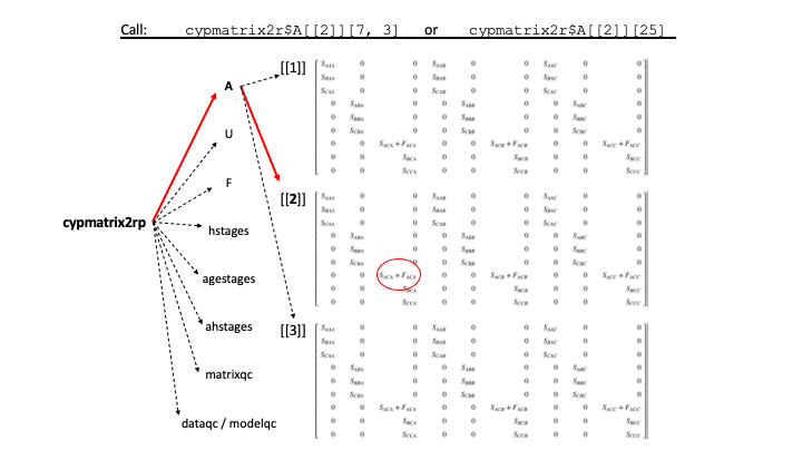
lefkoMat object, and how to call a specific element
Objects of class lefkoMat have their own summary() statements, which we can use to understand more about them.
summary(cypmatrix2rp)
>
> This ahistorical lefkoMat object contains 15 matrices.
>
> Each matrix is square with 11 rows and columns, and a total of 121 elements.
> A total of 266 survival transitions were estimated, with 17.733 per matrix.
> A total of 70 fecundity transitions were estimated, with 4.667 per matrix.
> This lefkoMat object covers 1 population, 3 patches, and 5 time steps.
>
> The dataset contains a total of 74 unique individuals and 320 unique transitions.
>
> Survival probability sum check (each matrix represented by column in order):
>          [,1]  [,2]  [,3]  [,4]  [,5]  [,6]  [,7]  [,8]  [,9] [,10] [,11] [,12]
> Min.    0.000 0.000 0.000 0.000 0.000 0.000 0.050 0.050 0.000 0.050 0.000 0.000
> 1st Qu. 0.075 0.025 0.075 0.025 0.075 0.075 0.140 0.140 0.100 0.140 0.100 0.100
> Median  0.180 0.100 0.180 0.100 0.180 0.180 0.909 0.778 0.686 0.857 0.750 0.575
> Mean    0.457 0.361 0.471 0.328 0.417 0.464 0.631 0.611 0.530 0.631 0.562 0.523
> 3rd Qu. 0.955 0.769 1.000 0.592 0.781 1.000 1.000 1.000 0.955 1.000 1.000 1.000
> Max.    1.000 1.000 1.000 1.000 1.000 1.000 1.000 1.000 1.000 1.000 1.000 1.000
>         [,13] [,14] [,15]
> Min.    0.000 0.000 0.000
> 1st Qu. 0.075 0.075 0.100
> Median  0.180 0.180 0.750
> Mean    0.432 0.450 0.562
> 3rd Qu. 0.875 1.000 1.000
> Max.    1.000 1.000 1.000
>
>
> Stages without connections leading to the rest of the life cycle found in matrices: 1 2 3 4 5 6 9 11 12 13 14 15
We start off learning that 15 matrices were estimated, and we learn the dimensionality of those matrices. Next we see how many elements were actually estimated, both overall and per matrix (actually the number of non-zero elements), and the mean number of non-zero survival transitions and fecundity terms per matrix. This is followed by the number of populations, patches or subpopulations, and time steps covered by the MPM. Then we see the number of individuals and transitions the matrices are based on. It is typical for population ecologists to consider the total number of transitions in a dataset as a measure of the statistical power of a matrix, but the number of individuals is just as important because each transition that an individual experiences is dependent on the other transitions that it also experiences. The following portion of the summary shows us the range of survival probabilities of stages in the matrices, where the survival probabilities are calculated as column sums of each \(\mathbf{U}\) matrix. Since there are 15 matrices, there are 15 survival summaries. It is important to check to see that no stage survives outside the realm of possibility (i.e. no probability should be greater than 1.0 or lower than 0.0). Unusual stage survival probabilities will result in a warning as a part of the summary() output. Finally, this summary() function checks each matrix to see if there are stages that appear to be dead ends in terms of the flow of transitions, and we see that most matrices have such occurrences. Typically this means that there are zero transitions due to a lack of data, or an overparameterized life history model.
The input arguments for function rlefko2() include patch = "all" and year = "all", but the function can be set to focus on any set of patches / subpopulations or years included within the data. Package lefko3 includes a great deal of flexibility here, and can estimate many matrices covering all of the populations, patches, and years occurring in a specific dataset. For example, if we had wished to skip the patch divisions within the population and instead estimate only annual matrices at the population level, then we can eliminate the patch and patchcol options altogether from the input, as below.
cypmatrix2r <- rlefko2(data = cypraw_v1, stageframe = cypframe_raw,
  year = "all", stages = c("stage3", "stage2"),
  size = c("size3added", "size2added"), supplement = cypsupp2_raw,
  yearcol = "year2", indivcol = "individ")

summary(cypmatrix2r)
>
> This ahistorical lefkoMat object contains 5 matrices.
>
> Each matrix is square with 11 rows and columns, and a total of 121 elements.
> A total of 120 survival transitions were estimated, with 24 per matrix.
> A total of 40 fecundity transitions were estimated, with 8 per matrix.
> This lefkoMat object covers 1 population, 1 patch, and 5 time steps.
>
> The dataset contains a total of 74 unique individuals and 320 unique transitions.
>
> Survival probability sum check (each matrix represented by column in order):
>          [,1]  [,2]  [,3]  [,4]  [,5]
> Min.    0.000 0.050 0.050 0.000 0.050
> 1st Qu. 0.100 0.140 0.140 0.100 0.140
> Median  0.689 0.870 0.864 0.610 0.882
> Mean    0.552 0.629 0.629 0.528 0.627
> 3rd Qu. 1.000 1.000 1.000 0.960 1.000
> Max.    1.000 1.000 1.000 1.000 1.000
>
>
> Stages without connections leading to the rest of the life cycle found in matrices: 1 4
Notice the difference in the output. The first call to rlefko2() yielded 15 matrices, because there are three patches and a total of six years of data, yielding five transitions between years (also referred to as time steps or periods). So, there were \(3 \times 5 = 15\) matrices. But in the second call, we no longer recognized patches and so have only estimated one set of five matrices covering the whole population. A further impact of this change is that the mean number of elements estimated per matrix increased, because there are fewer missing transitions in the dataset per matrix when the data are not parsed by patch. Finally, because the data are parsed across fewer matrices, we find fewer matrices with dead end stages. We can also create MPMs for specific patches and specific sets of years, setting the options appropriately.
Let’s try another exercise. This time, we will estimate matrices at the patch level, but only for the years 2006 and 2007. This will result in six matrices, since there are three patches and two monitoring occasions (note that focusing on years 2006 and 2007 means that we will only build matrices in which these are the years in time t).
cypmatrix2rp67 <- rlefko2(data = cypraw_v1, stageframe = cypframe_raw,
  year = c(2006, 2007), patch = "all", stages = c("stage3", "stage2"),
  size = c("size3added", "size2added"), supplement = cypsupp2_raw,
  yearcol = "year2", patchcol = "patchid", indivcol = "individ")

summary(cypmatrix2rp67)
>
> This ahistorical lefkoMat object contains 6 matrices.
>
> Each matrix is square with 11 rows and columns, and a total of 121 elements.
> A total of 111 survival transitions were estimated, with 18.5 per matrix.
> A total of 22 fecundity transitions were estimated, with 3.667 per matrix.
> This lefkoMat object covers 1 population, 3 patches, and 2 time steps.
>
> The dataset contains a total of 74 unique individuals and 320 unique transitions.
>
> Survival probability sum check (each matrix represented by column in order):
>          [,1]  [,2]  [,3]  [,4]  [,5]  [,6]
> Min.    0.000 0.000 0.050 0.000 0.000 0.000
> 1st Qu. 0.075 0.025 0.140 0.100 0.075 0.075
> Median  0.180 0.100 0.778 0.686 0.180 0.180
> Mean    0.471 0.328 0.611 0.530 0.432 0.450
> 3rd Qu. 1.000 0.592 1.000 0.955 0.875 1.000
> Max.    1.000 1.000 1.000 1.000 1.000 1.000
>
>
> Stages without connections leading to the rest of the life cycle found in matrices: 1 2 4 5 6
Finally, we will build matrices only for the years 2006 and 2007 in patch A. We expect only two matrices.
cypmatrix2rA67 <- rlefko2(data = cypraw_v1, stageframe = cypframe_raw,
  year = c(2006, 2007), patch = "A", stages = c("stage3", "stage2"),
  size = c("size3added", "size2added"), supplement = cypsupp2_raw,
  yearcol = "year2", patchcol = "patchid", indivcol = "individ")

summary(cypmatrix2rA67)
>
> This ahistorical lefkoMat object contains 2 matrices.
>
> Each matrix is square with 11 rows and columns, and a total of 121 elements.
> A total of 30 survival transitions were estimated, with 15 per matrix.
> A total of 0 fecundity transitions were estimated, with 0 per matrix.
> This lefkoMat object covers 1 population, 1 patch, and 2 time steps.
>
> The dataset contains a total of 74 unique individuals and 320 unique transitions.
>
> Survival probability sum check (each matrix represented by column in order):
>          [,1]  [,2]
> Min.    0.000 0.000
> 1st Qu. 0.075 0.025
> Median  0.180 0.100
> Mean    0.471 0.328
> 3rd Qu. 1.000 0.592
> Max.    1.000 1.000
>
>
> Stages without connections leading to the rest of the life cycle found in matrices: 1 2
This output is also interesting because it showcases one of the weaknesses of the raw MPM approach. We see that no individuals produced any offspring in patch A over these two time steps, so no non-zero fecundity terms were estimated. While this is a very accurate result, it can lead to problems if we think of the MPM as reflecting the underlying biology of the species. In this case, fecundity is missing most likely because there were too few individuals in this patch at these times and none of those present produced flowers. So, the luck of the draw prevented us from estimating some biologically important elements.
4.2 Ahistorical vs. historical matrix models
The matrices that we have built so far are all examples of raw ahistorical MPMs (ahMPMs). These are projection models in which the future stage of an individual is dependent only on its current stage, and not on previous stages. In other words, individual history is not incorporated into ahMPMs. It may seem odd that individual history is not incorporated into the matrices given that demographic datasets are composed of records of individual histories spanning several or even many monitoring occasions. However, construction of an ahMPM breaks up these individual histories into pairs of consecutive stages across time, with each stage-pair treated as independent of every other pair of consecutive stages. For example, if an individual is in stage A in occasion 1, stage B in occasion 2, stage E in occasion 3, and dead in occasion 4, then its individual history is broken up into three transitions: A-B, B-E, and E-Dead. Each of these transitions is assumed to be independent. The resulting projection matrix would be the same if these transitions originated from different individuals or the same one - their order and relationships do not have any impacts in ahMPM construction.
The independence of consecutive stage-pairs reflects a central assumption in ahMPM analysis: the stage of an individual in the next occasion is influenced only by its current stage. Conceptually, if an organism’s stage in the next occasion is entirely determined by its current stage, then its previous states do not influence these transitions. Thus, standard ahMPMs are two dimensional and reflect only the current and next immediate stage of individuals, given by the columns and rows, respectively. This is ultimately an extension of the iid assumption in statistics - that the states of individuals are independent and originate from identically-distributed random variables. This assumption helped make matrix projection models relatively easy to estimate even before the advent of personal computers.
The first MPMs were produced in the 1940s, with Leslie’s introduction of the age-structured model (Leslie 1945; Caswell 2001). We have never done a meta-analysis of all of these studies, but nonetheless it is safe to say that studies considering individual history are rare. The typical MPM study involves only ahMPMs, and so assumes independence of stage transitions across time even from the same individual. In fact, at the time of writing, we are aware of only five examples of studies breaking these assumptions and using a historical approach, in which some degree of individual history is incorporated into matrix estimation and analysis (Ehrlén 2000; Shefferson et al. 2014, 2017, 2018; deVries & Caswell 2018).
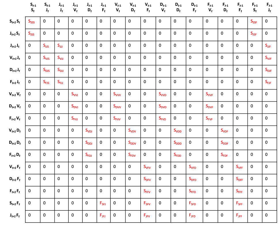
The historical MPM (hMPM) is an extension of the matrix projection model that incorporates information on one previous occasion into the determination of vital rates. Thus, the expected survival-transition probability of an individual in stage \(j\) in occasion t to stage \(k\) in occasion t+1 depends not only on its stage in occasion t but also on its stage in occasion t-1. Population ecologists considering this problem analytically might be inclined to add an extra dimension to the matrix to deal with this, thus creating a 3d array or cube. However, this is mathematically intractable, with many analyses becoming impossible (deVries & Caswell 2018). Instead, we utilize the approach developed by Ehrlén (2000), in which rows and columns represent life history stages paired in consecutive occasions. Thus, columns now represent the From pair of stages (stages in occasions t-1 and t), and rows now represent the To pair of stages (stages in occasions t and t+1), as in figure 4.3. This model is equivalent to the second-order model proposed by deVries & Caswell (2018), although the latter takes a different approach to parameterizing history in transitions involving individuals just born (we explain the difference further in this vignette).
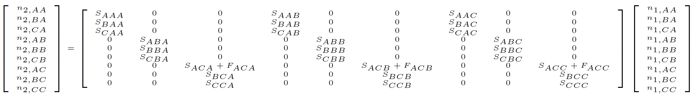
Historical MPMs can be projected forward in the same way as ahMPMs. In figure 4.4 we see an example of a projection one time step forward using the hMPM shown in figure 4.3.
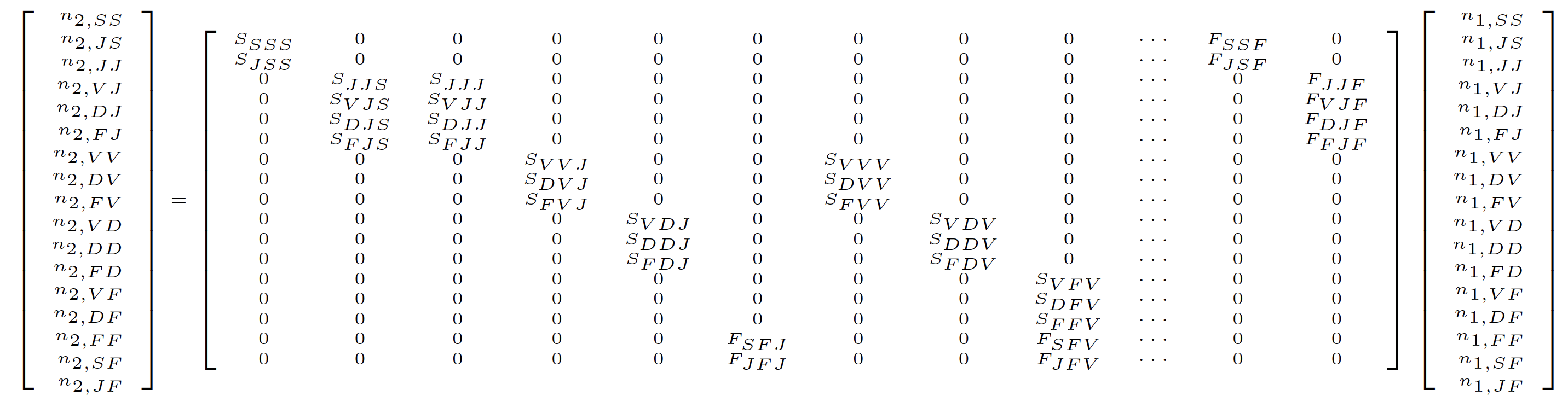
Here, \(n _{1,SS}\) is the number of individuals that were in stage \(S\) in both occasions 0 and 1, and \(n _{2,DF}\) is the number of individuals that were in stage \(D\) in occasion 2 and stage \(F\) in occasion 1.
Ahistorical matrices and historical matrices can be derived from the same datasets provided that individual fates are noted for three consecutive times each. We can refer to matrix elements as \(a _{kjl}\), where the element represents the rate at which individuals transition to stage \(k\) in occasion t+1 after having been in stage \(j\) in occasion t and in stage \(l\) in occasion t-1. If \(n _{kjl}\) is the number of individuals making this transition, \(n _{.jl}\) is the total number of individuals in stage \(j\) in occasion t and stage \(l\) in occasion t-1 regardless of stage or even status as alive or dead in occasion t+1, \(m\) is the number of stages in the life history model, and \(d\) is the number of stages plus death in the life history model (so that \(d=m+1\)), then we have the following equation.
\[\begin{equation} a _{kjl} = \frac{n _{kjl}}{n _{.jl}} = \frac{n _{kjl}}{\sum_{i=1}^{d} n _{ijl}} \tag{4.5} \end{equation}\]
Although we can use the actual numbers of individuals making historical transitions to estimate ahistorical MPMs, we cannot use the matrix elements in a historical MPM to calculate the associated ahistorical MPM elements, nor can we use the elements in an ahistorical MPM to calculate the elements in a historical MPM. This is due to the fact that historical transitions must be weighted by the numbers of individuals in each previous stage in occasions t and t-1 (\(n _{.jl}\)) to produce the proper ahistorical transition rates. Historical matrix elements contain no information about these weights. Thus, we have the following relationships between ahistorical survival-transition terms and the historical datasets.
\[\begin{equation} a _{kj} = \frac{\sum_{l=1}^{m} n _{kjl}}{\sum_{l=1}^{m} \sum_{i=1}^{d} n _{ijl}} \tag{4.6} \end{equation}\]
Historical MPMs normally require a much larger number of elements to be parameterized than ahMPMs do. Figure 4.3 illustrates this issue. Typically, a historical matrix has dimensions equal to the number of stages squared (although this may sometimes be reduced, if certain conditions are met). However, most of the increase in matrix elements is in structural zeros. In an ahistorical matrix, the only true zeros will be those elements corresponding to biologically impossible transitions, or those elements without any individuals taking the respective transition in a given time step. However, most elements in a historical MPM are structural zeros, because transition elements in hMPMs are only estimable if stage in occasion t is equal in the column and row stage pairs. For example, the transition probability between stage A in occasion t-1 and stage B in occasion t (column stage-pair), to stage C in occasion t and stage D in occasion t+1 (row stage-pair) equals 0, because an organism cannot be in both stages B and C in occasion t. Increasing the number of stages in the life history model causes these structural zeros to increase at a faster rate than the rate at which the number of truly estimable elements increases. In fact, if there are \(m\) stages in a life history, yielding \(m ^{2}\) elements in an ahistorical matrix, then although there will be \(m ^{4}\) elements in the historical matrix, only \(m^{3}\) will be potentially estimable while \((m-1) m^{3}\) will be structural zeros (we say potentially because some of the logically possible transitions may still be biologically impossible, or may have no data to yield values other than 0).
4.2.1 Historical MPMs in lefko3
Let’s build our first historical MPM with the Cypripedium candidum data. As before, we will build our MPM to cover all years and all patches.
cypmatrix3rp <- rlefko3(data = cypraw_v1, stageframe = cypframe_raw,
  year = "all", patch = "all", stages = c("stage3", "stage2", "stage1"),
  size = c("size3added", "size2added", "size1added"), supplement = cypsupp3_raw,
  yearcol = "year2", patchcol = "patchid", indivcol = "individ")

summary(cypmatrix3rp)
>
> This historical lefkoMat object contains 12 matrices.
>
> Each matrix is square with 121 rows and columns, and a total of 14641 elements.
> A total of 516 survival transitions were estimated, with 43 per matrix.
> A total of 70 fecundity transitions were estimated, with 5.833 per matrix.
> This lefkoMat object covers 1 population, 3 patches, and 4 time steps.
>
> The dataset contains a total of 74 unique individuals and 320 unique transitions.
>
> Survival probability sum check (each matrix represented by column in order):
>          [,1]   [,2]   [,3]  [,4]  [,5]  [,6] [,7]  [,8]  [,9]  [,10] [,11]
> Min.    0.000 0.0000 0.0000 0.000 0.000 0.000 0.00 0.000 0.000 0.0000 0.000
> 1st Qu. 0.000 0.0000 0.0000 0.000 0.000 0.000 0.00 0.000 0.000 0.0000 0.000
> Median  0.000 0.0000 0.0000 0.000 0.000 0.000 0.00 0.000 0.000 0.0000 0.000
> Mean    0.107 0.0945 0.0851 0.101 0.158 0.158 0.14 0.169 0.119 0.0851 0.119
> 3rd Qu. 0.000 0.0000 0.0000 0.000 0.100 0.100 0.05 0.100 0.000 0.0000 0.000
> Max.    1.000 1.0000 1.0000 1.000 1.000 1.000 1.00 1.000 1.000 1.0000 1.000
>         [,12]
> Min.    0.000
> 1st Qu. 0.000
> Median  0.000
> Mean    0.144
> 3rd Qu. 0.000
> Max.    1.000
>
>
> Stage-pairs without connections leading to the rest of the life cycle found in matrices: 1 2 3 4 5 6 7 8 9 10 11 12
Quickly scanning this output shows a number of differences relative to the ahMPM. First, there are three fewer matrices here than in the ahistorical case. There are three patches that we are estimating matrices for, and six years of data for each patch, leading to five possible ahistorical time steps and 15 possible ahistorical matrices. Since historical matrices require three years of transition data, only four historical transitions are possible per patch, leading to 12 total historical matrices. Second, the size of the matrices in terms of the number of rows and columns is the square of the dimensions of the ahistorical matrices. This leads to vastly more matrix elements within each matrix, although it turns out that most of these matrix elements are structural zeros because they reflect impossible transitions. Indeed, in this case, although there are 14,641 elements in each matrix, on average only 48.83 are actually estimated to values greater than 0.
Let’s look at the first matrix, corresponding to the transition from 2004 and 2005 to 2006 in the first patch (patch A, according to the labels element). Because this is a huge matrix, we will only look at the top corner, followed by a section toward the middle. Particularly note the sparseness - most elements are zeros, because most transitions are actually impossible. These matrices may also be exported to Microsoft Excel, Apple Numbers, or another spreadsheet program to look over in greater detail.
cypmatrix3rp$A[[1]][1:20,1:10]
>       [,1] [,2] [,3] [,4] [,5] [,6] [,7] [,8] [,9] [,10]
>  [1,] 0.08  0.0    0    0    0    0    0    0    0     0
>  [2,] 0.10  0.0    0    0    0    0    0    0    0     0
>  [3,] 0.00  0.0    0    0    0    0    0    0    0     0
>  [4,] 0.00  0.0    0    0    0    0    0    0    0     0
>  [5,] 0.00  0.0    0    0    0    0    0    0    0     0
>  [6,] 0.00  0.0    0    0    0    0    0    0    0     0
>  [7,] 0.00  0.0    0    0    0    0    0    0    0     0
>  [8,] 0.00  0.0    0    0    0    0    0    0    0     0
>  [9,] 0.00  0.0    0    0    0    0    0    0    0     0
> [10,] 0.00  0.0    0    0    0    0    0    0    0     0
> [11,] 0.00  0.0    0    0    0    0    0    0    0     0
> [12,] 0.00  0.0    0    0    0    0    0    0    0     0
> [13,] 0.00  0.0    0    0    0    0    0    0    0     0
> [14,] 0.00  0.1    0    0    0    0    0    0    0     0
> [15,] 0.00  0.0    0    0    0    0    0    0    0     0
> [16,] 0.00  0.0    0    0    0    0    0    0    0     0
> [17,] 0.00  0.0    0    0    0    0    0    0    0     0
> [18,] 0.00  0.0    0    0    0    0    0    0    0     0
> [19,] 0.00  0.0    0    0    0    0    0    0    0     0
> [20,] 0.00  0.0    0    0    0    0    0    0    0     0
print(cypmatrix3rp$A[[1]][66:85,73:81], digits = 3)
>          [,1]     [,2] [,3] [,4] [,5] [,6] [,7] [,8] [,9]
>  [1,]   0.000    0.000    0    0    0    0    0    0    0
>  [2,] 357.143    0.000    0    0    0    0    0    0    0
>  [3,] 357.143    0.000    0    0    0    0    0    0    0
>  [4,]   0.000    0.000    0    0    0    0    0    0    0
>  [5,]   0.000    0.000    0    0    0    0    0    0    0
>  [6,]   0.000    0.000    0    0    0    0    0    0    0
>  [7,]   0.143    0.000    0    0    0    0    0    0    0
>  [8,]   0.714    0.000    0    0    0    0    0    0    0
>  [9,]   0.000    0.000    0    0    0    0    0    0    0
> [10,]   0.000    0.000    0    0    0    0    0    0    0
> [11,]   0.000    0.000    0    0    0    0    0    0    0
> [12,]   0.000    0.000    0    0    0    0    0    0    0
> [13,]   0.000 1666.667    0    0    0    0    0    0    0
> [14,]   0.000 1666.667    0    0    0    0    0    0    0
> [15,]   0.000    0.000    0    0    0    0    0    0    0
> [16,]   0.000    0.000    0    0    0    0    0    0    0
> [17,]   0.000    0.000    0    0    0    0    0    0    0
> [18,]   0.000    0.000    0    0    0    0    0    0    0
> [19,]   0.000    0.667    0    0    0    0    0    0    0
> [20,]   0.000    0.333    0    0    0    0    0    0    0
As before, we can create matrices at the full population level by withholding the patch and patchcol options, as below.
cypmatrix3r <- rlefko3(data = cypraw_v1, stageframe = cypframe_raw,
  year = "all", stages = c("stage3", "stage2", "stage1"),
  size = c("size3added", "size2added", "size1added"), supplement = cypsupp3_raw,
  yearcol = "year2", indivcol = "individ")

summary(cypmatrix3r)
>
> This historical lefkoMat object contains 4 matrices.
>
> Each matrix is square with 121 rows and columns, and a total of 14641 elements.
> A total of 242 survival transitions were estimated, with 60.5 per matrix.
> A total of 54 fecundity transitions were estimated, with 13.5 per matrix.
> This lefkoMat object covers 1 population, 1 patch, and 4 time steps.
>
> The dataset contains a total of 74 unique individuals and 320 unique transitions.
>
> Survival probability sum check (each matrix represented by column in order):
>          [,1]  [,2]  [,3]  [,4]
> Min.    0.000 0.000 0.000 0.000
> 1st Qu. 0.000 0.000 0.000 0.000
> Median  0.000 0.000 0.000 0.000
> Mean    0.173 0.179 0.166 0.198
> 3rd Qu. 0.100 0.100 0.100 0.100
> Max.    1.000 1.000 1.000 1.000
>
>
> Stage-pairs without connections leading to the rest of the life cycle found in matrices: 1 2 3 4
We now have only four matrices, corresponding to the full population in each year at time t. Next, let’s focus only on years 2006 and 2007 in all patches, as before.
cypmatrix3rp67 <- rlefko3(data = cypraw_v1, stageframe = cypframe_raw,
  year = c(2006, 2007), patch = "all", stages = c("stage3", "stage2", "stage1"),
  size = c("size3added", "size2added", "size1added"), supplement = cypsupp3_raw,
  yearcol = "year2", patchcol = "patchid", indivcol = "individ")

summary(cypmatrix3rp67)
>
> This historical lefkoMat object contains 6 matrices.
>
> Each matrix is square with 121 rows and columns, and a total of 14641 elements.
> A total of 260 survival transitions were estimated, with 43.333 per matrix.
> A total of 30 fecundity transitions were estimated, with 5 per matrix.
> This lefkoMat object covers 1 population, 3 patches, and 2 time steps.
>
> The dataset contains a total of 74 unique individuals and 320 unique transitions.
>
> Survival probability sum check (each matrix represented by column in order):
>           [,1]   [,2]  [,3] [,4]   [,5]  [,6]
> Min.    0.0000 0.0000 0.000 0.00 0.0000 0.000
> 1st Qu. 0.0000 0.0000 0.000 0.00 0.0000 0.000
> Median  0.0000 0.0000 0.000 0.00 0.0000 0.000
> Mean    0.0945 0.0851 0.158 0.14 0.0851 0.119
> 3rd Qu. 0.0000 0.0000 0.100 0.05 0.0000 0.000
> Max.    1.0000 1.0000 1.000 1.00 1.0000 1.000
>
>
> Stage-pairs without connections leading to the rest of the life cycle found in matrices: 1 2 3 4 5 6
We find six matrices, corresponding to the years 2006 and 2007 for each of the three patches. And now let’s focus in on years 2006 and 2007 in the first patch, patch A.
cypmatrix3rA67 <- rlefko3(data = cypraw_v1, stageframe = cypframe_raw,
  year = c(2006, 2007), patch = "A", stages = c("stage3", "stage2", "stage1"),
  size = c("size3added", "size2added", "size1added"), supplement = cypsupp3_raw,
  yearcol = "year2", patchcol = "patchid", indivcol = "individ")

summary(cypmatrix3rA67)
>
> This historical lefkoMat object contains 2 matrices.
>
> Each matrix is square with 121 rows and columns, and a total of 14641 elements.
> A total of 78 survival transitions were estimated, with 39 per matrix.
> A total of 0 fecundity transitions were estimated, with 0 per matrix.
> This lefkoMat object covers 1 population, 1 patch, and 2 time steps.
>
> The dataset contains a total of 74 unique individuals and 320 unique transitions.
>
> Survival probability sum check (each matrix represented by column in order):
>           [,1]   [,2]
> Min.    0.0000 0.0000
> 1st Qu. 0.0000 0.0000
> Median  0.0000 0.0000
> Mean    0.0945 0.0851
> 3rd Qu. 0.0000 0.0000
> Max.    1.0000 1.0000
>
>
> Stage-pairs without connections leading to the rest of the life cycle found in matrices: 1 2
As before, we find no fecundity terms estimated, as no individuals in patch A were reproductive in these two times.
4.3 Alternate parameterizations of historical MPMs
deVries & Caswell (2018) details different approaches to the development of hMPMs, differing in how state or stage in occasion t-1 is incorporated into the matrix. Full prior stage dependence models deal with history by incorporating prior condition as the exact stage of an organism in occasion t-1, yielding 2d matrices showing stage pairs in occasion t-1 and t along the columns of the matrix, and stage pairs in occasion t and t+1 along the rows of the matrix. Prior condition models deal with history by making the transition from stage t to stage t+1 a function of stage at occasion t and condition in occasion t-1. Prior condition can be determined in the same way that current stage is determined (e.g. size classification), or a different measure of condition can be used, such as growth (i.e. the change in size between occasions t-1 and t).
One key feature proposed by deVries & Caswell (2018) is the addition of a stage to account for the prior status of newborn individuals. This reflects a different interpretation of the historical transition from Ehrlén (2000). In Ehrlén (2000), all matrix elements simply reflect the order of the events in a single transition, including both fecundity and survival-transition events. However, in deVries & Caswell (2018), these matrix elements must also reflect the history of specific individuals. In the latter case, the fact that a newborn in occasion t did not exist in occasion t-1 requires that a new prior stage is constructed and used in the matrix to account for that individual’s prior lack of existence. This new stage only exists in the prior occasion, and is only used for newborns in the first survival transition from birth. So, for example, in a historical MPM where the first stage is the newborn stage and only the third stage is reproductive, we add a fourth stage to the prior portion of the row and column. Thus, we may start with the following hMPM in Ehrlén (2000) format:
This hMPM becomes as follows in deVries & Caswell (2018) format, where the prior “pre-born” stage is shown as \(P\).
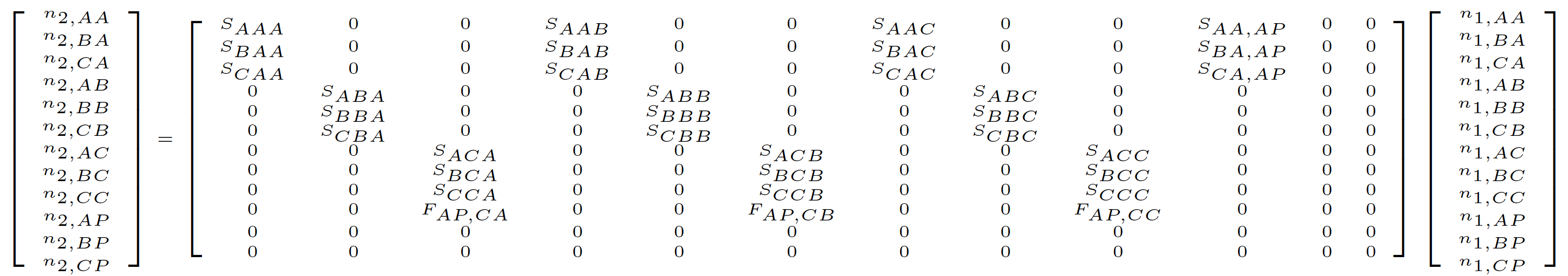
Package lefko3 generally implements the full prior stage dependence model approach, particularly in the development of raw matrices. However, in principle, function-based matrices developed with lefko3 can be seen as falling within the prior condition model approach where prior condition is determined in the same way as current stage. We also implement both the Ehrlén (2000) format and the deVries & Caswell (2018) format, and use the former as the default. We leave it to the user to decide which approach to use, and point out only that the literature suggests that maternal condition can have long-term effects on offspring survival, for example through maternal care and epigenetic influences (Descamps et al. 2008; Beamonte-Barrientos et al. 2010; Dogra & Dani 2019). Thus, retaining maternal state as the prior condition of a newborn makes some logical sense and has a basis in the literature.
Let’s build a deVries format hMPM for the Cypripedium candidum dataset.
cypmatrix3rp_dev <- rlefko3(data = cypraw_v1, stageframe = cypframe_raw,
  year = "all", patch = "all", stages = c("stage3", "stage2", "stage1"),
  size = c("size3added", "size2added", "size1added"), supplement = cypsupp3_raw,
  yearcol = "year2", patchcol = "patchid", indivcol = "individ",
  format = "deVries")

summary(cypmatrix3rp_dev)
>
> This historical lefkoMat object contains 12 matrices.
>
> Each matrix is square with 132 rows and columns, and a total of 17424 elements.
> A total of 516 survival transitions were estimated, with 43 per matrix.
> A total of 70 fecundity transitions were estimated, with 5.833 per matrix.
> This lefkoMat object covers 1 population, 3 patches, and 4 time steps.
>
> The dataset contains a total of 74 unique individuals and 320 unique transitions.
>
> Survival probability sum check (each matrix represented by column in order):
>           [,1]   [,2]  [,3]   [,4]  [,5]   [,6]  [,7]   [,8]  [,9] [,10] [,11]
> Min.    0.0000 0.0000 0.000 0.0000 0.000 0.0000 0.000 0.0000 0.000 0.000 0.000
> 1st Qu. 0.0000 0.0000 0.000 0.0000 0.000 0.0000 0.000 0.0000 0.000 0.000 0.000
> Median  0.0000 0.0000 0.000 0.0000 0.000 0.0000 0.000 0.0000 0.000 0.000 0.000
> Mean    0.0981 0.0866 0.078 0.0923 0.144 0.1445 0.128 0.1548 0.109 0.078 0.109
> 3rd Qu. 0.0000 0.0000 0.000 0.0000 0.000 0.0125 0.000 0.0125 0.000 0.000 0.000
> Max.    1.0000 1.0000 1.000 1.0000 1.000 1.0000 1.000 1.0000 1.000 1.000 1.000
>         [,12]
> Min.    0.000
> 1st Qu. 0.000
> Median  0.000
> Mean    0.132
> 3rd Qu. 0.000
> Max.    1.000
>
>
> Stage-pairs without connections leading to the rest of the life cycle found in matrices: 1 2 3 4 5 6 7 8 9 10 11 12
Our new matrices have 11 more rows and columns, and 2,783 more elements. To see what is different, compare the hstages element in each on your own, and you will see the inclusion of some new stage pairs with the AlmostBorn stage. It is also possible for some transitions to be split, occasionally yielding more transitions than were estimated in the Ehrlén format case.
4.4 Sparse matrix format
Historical matrices can be huge. Unfortunately, the larger a matrix is, the longer it takes to create and to analyze, and the greater the share of memory needed to deal with it. In fact, some MPMs can take up many gigabytes of memory, and such situations risk not only extending analysis time into unreasonable territory, but also analysis termination due to memory shortage. To help deal with these situations, all matrix creation functions in package lefko3 can produce and analyze MPMs in sparse matrix format. As an example, let’s create a sparse format version of the deVries-formatted historical MPM.
cypmatrix3rp_dev_sparse <- rlefko3(data = cypraw_v1, stageframe = cypframe_raw,
  year = "all", patch = "all", stages = c("stage3", "stage2", "stage1"),
  size = c("size3added", "size2added", "size1added"), supplement = cypsupp3_raw,
  yearcol = "year2", patchcol = "patchid", indivcol = "individ",
  format = "deVries", sparse_output = TRUE)

summary(cypmatrix3rp_dev_sparse)
>
> This historical lefkoMat object contains 12 matrices.
>
> Each matrix is square with 132 rows and columns, and a total of 17424 elements.
> A total of 516 survival transitions were estimated, with 43 per matrix.
> A total of 70 fecundity transitions were estimated, with 5.833 per matrix.
> This lefkoMat object covers 1 population, 3 patches, and 4 time steps.
>
> The dataset contains a total of 74 unique individuals and 320 unique transitions.
>
> Survival probability sum check (each matrix represented by column in order):
>           [,1]   [,2]  [,3]   [,4]  [,5]   [,6]  [,7]   [,8]  [,9] [,10] [,11]
> Min.    0.0000 0.0000 0.000 0.0000 0.000 0.0000 0.000 0.0000 0.000 0.000 0.000
> 1st Qu. 0.0000 0.0000 0.000 0.0000 0.000 0.0000 0.000 0.0000 0.000 0.000 0.000
> Median  0.0000 0.0000 0.000 0.0000 0.000 0.0000 0.000 0.0000 0.000 0.000 0.000
> Mean    0.0981 0.0866 0.078 0.0923 0.144 0.1445 0.128 0.1548 0.109 0.078 0.109
> 3rd Qu. 0.0000 0.0000 0.000 0.0000 0.000 0.0125 0.000 0.0125 0.000 0.000 0.000
> Max.    1.0000 1.0000 1.000 1.0000 1.000 1.0000 1.000 1.0000 1.000 1.000 1.000
>         [,12]
> Min.    0.000
> 1st Qu. 0.000
> Median  0.000
> Mean    0.132
> 3rd Qu. 0.000
> Max.    1.000
>
>
> Stage-pairs without connections leading to them found in matrices: 1 2 3 4 5 6 7 8 9 10 11 12
Looking over the output, it is clear that we have the same MPM. However, we see a difference in formatting when we actually zoom in to take a look at a specific matrix.
cypmatrix3rp_dev_sparse$A[[1]]
> 132 x 132 sparse Matrix of class "dgCMatrix"
>
>  [1,] 0.08 .   . . . . . . . . . . . . . . . . . . . . . . . . . . . . . . . ......
>  [2,] 0.10 .   . . . . . . . . . . . . . . . . . . . . . . . . . . . . . . . ......
>  [3,] .    .   . . . . . . . . . . . . . . . . . . . . . . . . . . . . . . . ......
>  [4,] .    .   . . . . . . . . . . . . . . . . . . . . . . . . . . . . . . . ......
>  [5,] .    .   . . . . . . . . . . . . . . . . . . . . . . . . . . . . . . . ......
>  [6,] .    .   . . . . . . . . . . . . . . . . . . . . . . . . . . . . . . . ......
>  [7,] .    .   . . . . . . . . . . . . . . . . . . . . . . . . . . . . . . . ......
>  [8,] .    .   . . . . . . . . . . . . . . . . . . . . . . . . . . . . . . . ......
>  [9,] .    .   . . . . . . . . . . . . . . . . . . . . . . . . . . . . . . . ......
> [10,] .    .   . . . . . . . . . . . . . . . . . . . . . . . . . . . . . . . ......
> [11,] .    .   . . . . . . . . . . . . . . . . . . . . . . . . . . . . . . . ......
> [12,] .    .   . . . . . . . . . . . . . . . . . . . . . . . . . . . . . . . ......
> [13,] .    .   . . . . . . . . . . . . . . . . . . . . . . . . . . . . . . . ......
> [14,] .    0.1 . . . . . . . . . . . . . . . . . . . . . . . . . . . . . . . ......
> [15,] .    .   . . . . . . . . . . . . . . . . . . . . . . . . . . . . . . . ......
>
>  ..............................
>  ........suppressing 99 columns and 102 rows in show(); maybe adjust options(max.print=, width=)
>  ..............................
>
> [118,] . . . . . . . . . . . . . . . . . . . . . . . . . . . . . . . . . ......
> [119,] . . . . . . . . . . . . . . . . . . . . . . . . . . . . . . . . . ......
> [120,] . . . . . . . . . . . . . . . . . . . . . . . . . . . . . . . . . ......
> [121,] . . . . . . . . . . . . . . . . . . . . . . . . . . . . . . . . . ......
> [122,] . . . . . . . . . . . . . . . . . . . . . . . . . . . . . . . . . ......
> [123,] . . . . . . . . . . . . . . . . . . . . . . . . . . . . . . . . . ......
> [124,] . . . . . . . . . . . . . . . . . . . . . . . . . . . . . . . . . ......
> [125,] . . . . . . . . . . . . . . . . . . . . . . . . . . . . . . . . . ......
> [126,] . . . . . . . . . . . . . . . . . . . . . . . . . . . . . . . . . ......
> [127,] . . . . . . . . . . . . . . . . . . . . . . . . . . . . . . . . . ......
> [128,] . . . . . . . . . . . . . . . . . . . . . . . . . . . . . . . . . ......
> [129,] . . . . . . . . . . . . . . . . . . . . . . . . . . . . . . . . . ......
> [130,] . . . . . . . . . . . . . . . . . . . . . . . . . . . . . . . . . ......
> [131,] . . . . . . . . . . . . . . . . . . . . . . . . . . . . . . . . . ......
> [132,] . . . . . . . . . . . . . . . . . . . . . . . . . . . . . . . . . ......
Users with recent versions of RStudio can see the amount of memory taken up by each of these MPMs. However, let’s see how much each object is taking up using the pryr package, as below (please install package pryr if it is not installed).
The standard matrix format version of the above MPM takes up roughly 5 MB on the author’s computer, while the sparse format MPM takes up only 80 kB. Clearly we have a serious savings in memory usage with the sparse format for historical MPMs.
The dgCMatrix sparse format is described in detail in package Matrix, and is a reliable sparse matrix format that retains compatibility with many other programming languages. We generally advocate the use of sparse format whenever a historical MPM with more than 40 stages is used, as well as in age-by-stage matrices in which the number of rows and columns is greater than 200 or so each. However, sparse format should not be used for most ahistorical IPMs, since they are inherently dense and will take up more memory than the equivalent IPM in standard matrix format.
4.5 Matrix reduction
One important issue that arises in raw MPM and hMPM estimation is that some rows and columns may have only zeroes associated with them. This is particularly the case with raw hMPMs, since these are quite data-hungry MPMs. Sometimes all of the rows and columns associated with a particular stage pair are completely full of zeros, because individuals were not observed to take particular transitions related to those stage pairs. In these situations, matrices can be reduced by eliminating the stage-pair or stage altogether. The result is a set of smaller matrices, which is useful considering that historical MPMs are generally large and can take up a great deal of memory. We can tell R to develop reduced MPMs by using the reduce = TRUE option in the matrix generating function that we are using. Note that this option is available in all matrix generating functions, even for those creating ahistorical MPMs, and that rows and columns will be reduced only if all matrices within the lefkoMat object being produced have empty rows and columns associated with a particular stage or stage-pair.
cypmatrix3rp_red <- rlefko3(data = cypraw_v1, stageframe = cypframe_raw,
  year = "all", patch = "all", stages = c("stage3", "stage2", "stage1"),
  size = c("size3added", "size2added", "size1added"), supplement = cypsupp3_raw,
  yearcol = "year2", patchcol = "patchid", indivcol = "individ",
  reduce = TRUE)

summary(cypmatrix3rp_red)
>
> This historical lefkoMat object contains 12 matrices.
>
> Each matrix is square with 43 rows and columns, and a total of 1849 elements.
> A total of 516 survival transitions were estimated, with 43 per matrix.
> A total of 70 fecundity transitions were estimated, with 5.833 per matrix.
> This lefkoMat object covers 1 population, 3 patches, and 4 time steps.
>
> The dataset contains a total of 74 unique individuals and 320 unique transitions.
>
> Survival probability sum check (each matrix represented by column in order):
>          [,1]  [,2]  [,3]  [,4]  [,5]  [,6]  [,7]  [,8]  [,9] [,10] [,11] [,12]
> Min.    0.000 0.000 0.000 0.000 0.000 0.000 0.000 0.000 0.000 0.000 0.000 0.000
> 1st Qu. 0.000 0.000 0.000 0.000 0.025 0.075 0.000 0.075 0.000 0.000 0.000 0.000
> Median  0.100 0.100 0.100 0.100 0.200 0.200 0.200 0.200 0.100 0.100 0.100 0.180
> Mean    0.301 0.266 0.239 0.283 0.443 0.443 0.393 0.475 0.336 0.239 0.336 0.405
> 3rd Qu. 0.650 0.200 0.200 0.475 1.000 1.000 1.000 1.000 0.875 0.200 0.875 1.000
> Max.    1.000 1.000 1.000 1.000 1.000 1.000 1.000 1.000 1.000 1.000 1.000 1.000
>
>
> Stage-pairs without connections leading to the rest of the life cycle found in matrices: 1 2 3 4 5 6 7 8 9 10 11 12
Our new hMPM has matrices with 43 rows and columns, while the original unreduced hMPM has matrices with 121 rows and columns. This is a reduction of 78 rows and columns, with an overall reduction in the size of the matrix by \(14641-1849 = 12792\) elements. This should speed up later calculations greatly.
4.6 Arithmetic mean matrices
Now that we have created our MPMs, we might wish to create element-wise arithmetic mean matrices to aid inference and further analysis. For example, we might be interested in developing patch-level means and an overall population mean, but one in which the element means weight each patch and each year equally. For this purpose, we can use the lmean() function. Let’s take a look at the element-wise mean raw ahMPM first.
cyp2rp_mean <- lmean(cypmatrix2rp)
cyp2rp_mean
> $A
> $A[[1]]
> [,1] [,2] [,3] [,4] [,5] [,6] [,7] [,8]
> [1,] 0.08 0.0 0.0 0.00 0.00000000 0.00000000 62.50000000 422.22222222
> [2,] 0.10 0.0 0.0 0.00 0.00000000 0.00000000 62.50000000 422.22222222
> [3,] 0.00 0.1 0.0 0.00 0.00000000 0.00000000 0.00000000 0.00000000
> [4,] 0.00 0.0 0.1 0.00 0.00000000 0.00000000 0.00000000 0.00000000
> [5,] 0.00 0.0 0.0 0.05 0.05000000 0.00000000 0.00000000 0.00000000
> [6,] 0.00 0.0 0.0 0.00 0.04083333 0.00000000 0.05833333 0.04444444
> [7,] 0.00 0.0 0.0 0.00 0.41964646 0.06666667 0.59949495 0.19555556
> [8,] 0.00 0.0 0.0 0.00 0.14707071 0.33333333 0.21010101 0.59555556
> [9,] 0.00 0.0 0.0 0.00 0.00000000 0.00000000 0.00000000 0.08444444
> [10,] 0.00 0.0 0.0 0.00 0.00000000 0.00000000 0.00000000 0.00000000
> [11,] 0.00 0.0 0.0 0.00 0.00000000 0.00000000 0.00000000 0.00000000
> [,9] [,10] [,11]
> [1,] 1.583333e+03 0.0 0
> [2,] 1.583333e+03 0.0 0
> [3,] 0.000000e+00 0.0 0
> [4,] 0.000000e+00 0.0 0
> [5,] 0.000000e+00 0.0 0
> [6,] 0.000000e+00 0.0 0
> [7,] 6.666667e-02 0.0 0
> [8,] 2.500000e-01 0.2 0
> [9,] 4.833333e-01 0.0 0
> [10,] 2.000000e-01 0.0 0
> [11,] 0.000000e+00 0.0 0
>
> $A[[2]]
> [,1] [,2] [,3] [,4] [,5] [,6] [,7] [,8]
> [1,] 0.08 0.0 0.0 0.00 0.00000000 0.00000000 55.55555556 572.91666667
> [2,] 0.10 0.0 0.0 0.00 0.00000000 0.00000000 55.55555556 572.91666667
> [3,] 0.00 0.1 0.0 0.00 0.00000000 0.00000000 0.00000000 0.00000000
> [4,] 0.00 0.0 0.1 0.00 0.00000000 0.00000000 0.00000000 0.00000000
> [5,] 0.00 0.0 0.0 0.05 0.05000000 0.00000000 0.00000000 0.00000000
> [6,] 0.00 0.0 0.0 0.00 0.05373737 0.06666667 0.07676768 0.05416667
> [7,] 0.00 0.0 0.0 0.00 0.32181818 0.46666667 0.45974026 0.23083333
> [8,] 0.00 0.0 0.0 0.00 0.21676768 0.20000000 0.30966811 0.50166667
> [9,] 0.00 0.0 0.0 0.00 0.00000000 0.00000000 0.02222222 0.14416667
> [10,] 0.00 0.0 0.0 0.00 0.00000000 0.06666667 0.02222222 0.01250000
> [11,] 0.00 0.0 0.0 0.00 0.00000000 0.00000000 0.00000000 0.00000000
> [,9] [,10] [,11]
> [1,] 2392.8571429 2875.0 6e+03
> [2,] 2392.8571429 2875.0 6e+03
> [3,] 0.0000000 0.0 0e+00
> [4,] 0.0000000 0.0 0e+00
> [5,] 0.0000000 0.0 0e+00
> [6,] 0.0000000 0.0 0e+00
> [7,] 0.0500000 0.0 0e+00
> [8,] 0.4000000 0.1 0e+00
> [9,] 0.3428571 0.2 0e+00
> [10,] 0.2071429 0.6 2e-01
> [11,] 0.0000000 0.1 4e-01
>
> $A[[3]]
> [,1] [,2] [,3] [,4] [,5] [,6] [,7] [,8] [,9]
> [1,] 0.08 0.0 0.0 0.00 0.00000000 0.0 0.00000000 422.61904762 1625.0000000
> [2,] 0.10 0.0 0.0 0.00 0.00000000 0.0 0.00000000 422.61904762 1625.0000000
> [3,] 0.00 0.1 0.0 0.00 0.00000000 0.0 0.00000000 0.00000000 0.0000000
> [4,] 0.00 0.0 0.1 0.00 0.00000000 0.0 0.00000000 0.00000000 0.0000000
> [5,] 0.00 0.0 0.0 0.05 0.05000000 0.0 0.00000000 0.00000000 0.0000000
> [6,] 0.00 0.0 0.0 0.00 0.04666667 0.0 0.06666667 0.03333333 0.0000000
> [7,] 0.00 0.0 0.0 0.00 0.35000000 0.1 0.50000000 0.11666667 0.1333333
> [8,] 0.00 0.0 0.0 0.00 0.18666667 0.1 0.26666667 0.54761905 0.3333333
> [9,] 0.00 0.0 0.0 0.00 0.00000000 0.0 0.06666667 0.22380952 0.5333333
> [10,] 0.00 0.0 0.0 0.00 0.00000000 0.0 0.00000000 0.07857143 0.0000000
> [11,] 0.00 0.0 0.0 0.00 0.00000000 0.0 0.00000000 0.00000000 0.0000000
> [,10] [,11]
> [1,] 750.0 2500.0
> [2,] 750.0 2500.0
> [3,] 0.0 0.0
> [4,] 0.0 0.0
> [5,] 0.0 0.0
> [6,] 0.0 0.0
> [7,] 0.0 0.0
> [8,] 0.1 0.0
> [9,] 0.2 0.0
> [10,] 0.4 0.2
> [11,] 0.1 0.4
>
> $A[[4]]
> [,1] [,2] [,3] [,4] [,5] [,6] [,7] [,8]
> [1,] 0.08 0.0 0.0 0.00 0.00000000 0.00000000 39.351851852 472.58597884
> [2,] 0.10 0.0 0.0 0.00 0.00000000 0.00000000 39.351851852 472.58597884
> [3,] 0.00 0.1 0.0 0.00 0.00000000 0.00000000 0.000000000 0.00000000
> [4,] 0.00 0.0 0.1 0.00 0.00000000 0.00000000 0.000000000 0.00000000
> [5,] 0.00 0.0 0.0 0.05 0.05000000 0.00000000 0.000000000 0.00000000
> [6,] 0.00 0.0 0.0 0.00 0.04707912 0.02222222 0.067255892 0.04398148
> [7,] 0.00 0.0 0.0 0.00 0.36382155 0.21111111 0.519745070 0.18101852
> [8,] 0.00 0.0 0.0 0.00 0.18350168 0.21111111 0.262145262 0.54828042
> [9,] 0.00 0.0 0.0 0.00 0.00000000 0.00000000 0.029629630 0.15080688
> [10,] 0.00 0.0 0.0 0.00 0.00000000 0.02222222 0.007407407 0.03035714
> [11,] 0.00 0.0 0.0 0.00 0.00000000 0.00000000 0.000000000 0.00000000
> [,9] [,10] [,11]
> [1,] 1.867063e+03 1.208333e+03 2833.3333333
> [2,] 1.867063e+03 1.208333e+03 2833.3333333
> [3,] 0.000000e+00 0.000000e+00 0.0000000
> [4,] 0.000000e+00 0.000000e+00 0.0000000
> [5,] 0.000000e+00 0.000000e+00 0.0000000
> [6,] 0.000000e+00 0.000000e+00 0.0000000
> [7,] 8.333333e-02 0.000000e+00 0.0000000
> [8,] 3.277778e-01 1.333333e-01 0.0000000
> [9,] 4.531746e-01 1.333333e-01 0.0000000
> [10,] 1.357143e-01 3.333333e-01 0.1333333
> [11,] 0.000000e+00 6.666667e-02 0.2666667
>
>
> $U
> $U[[1]]
> [,1] [,2] [,3] [,4] [,5] [,6] [,7] [,8]
> [1,] 0.08 0.0 0.0 0.00 0.00000000 0.00000000 0.00000000 0.00000000
> [2,] 0.10 0.0 0.0 0.00 0.00000000 0.00000000 0.00000000 0.00000000
> [3,] 0.00 0.1 0.0 0.00 0.00000000 0.00000000 0.00000000 0.00000000
> [4,] 0.00 0.0 0.1 0.00 0.00000000 0.00000000 0.00000000 0.00000000
> [5,] 0.00 0.0 0.0 0.05 0.05000000 0.00000000 0.00000000 0.00000000
> [6,] 0.00 0.0 0.0 0.00 0.04083333 0.00000000 0.05833333 0.04444444
> [7,] 0.00 0.0 0.0 0.00 0.41964646 0.06666667 0.59949495 0.19555556
> [8,] 0.00 0.0 0.0 0.00 0.14707071 0.33333333 0.21010101 0.59555556
> [9,] 0.00 0.0 0.0 0.00 0.00000000 0.00000000 0.00000000 0.08444444
> [10,] 0.00 0.0 0.0 0.00 0.00000000 0.00000000 0.00000000 0.00000000
> [11,] 0.00 0.0 0.0 0.00 0.00000000 0.00000000 0.00000000 0.00000000
> [,9] [,10] [,11]
> [1,] 0.00000000 0.0 0
> [2,] 0.00000000 0.0 0
> [3,] 0.00000000 0.0 0
> [4,] 0.00000000 0.0 0
> [5,] 0.00000000 0.0 0
> [6,] 0.00000000 0.0 0
> [7,] 0.06666667 0.0 0
> [8,] 0.25000000 0.2 0
> [9,] 0.48333333 0.0 0
> [10,] 0.20000000 0.0 0
> [11,] 0.00000000 0.0 0
>
> $U[[2]]
> [,1] [,2] [,3] [,4] [,5] [,6] [,7] [,8] [,9]
> [1,] 0.08 0.0 0.0 0.00 0.00000000 0.00000000 0.00000000 0.00000000 0.0000000
> [2,] 0.10 0.0 0.0 0.00 0.00000000 0.00000000 0.00000000 0.00000000 0.0000000
> [3,] 0.00 0.1 0.0 0.00 0.00000000 0.00000000 0.00000000 0.00000000 0.0000000
> [4,] 0.00 0.0 0.1 0.00 0.00000000 0.00000000 0.00000000 0.00000000 0.0000000
> [5,] 0.00 0.0 0.0 0.05 0.05000000 0.00000000 0.00000000 0.00000000 0.0000000
> [6,] 0.00 0.0 0.0 0.00 0.05373737 0.06666667 0.07676768 0.05416667 0.0000000
> [7,] 0.00 0.0 0.0 0.00 0.32181818 0.46666667 0.45974026 0.23083333 0.0500000
> [8,] 0.00 0.0 0.0 0.00 0.21676768 0.20000000 0.30966811 0.50166667 0.4000000
> [9,] 0.00 0.0 0.0 0.00 0.00000000 0.00000000 0.02222222 0.14416667 0.3428571
> [10,] 0.00 0.0 0.0 0.00 0.00000000 0.06666667 0.02222222 0.01250000 0.2071429
> [11,] 0.00 0.0 0.0 0.00 0.00000000 0.00000000 0.00000000 0.00000000 0.0000000
> [,10] [,11]
> [1,] 0.0 0.0
> [2,] 0.0 0.0
> [3,] 0.0 0.0
> [4,] 0.0 0.0
> [5,] 0.0 0.0
> [6,] 0.0 0.0
> [7,] 0.0 0.0
> [8,] 0.1 0.0
> [9,] 0.2 0.0
> [10,] 0.6 0.2
> [11,] 0.1 0.4
>
> $U[[3]]
> [,1] [,2] [,3] [,4] [,5] [,6] [,7] [,8] [,9] [,10]
> [1,] 0.08 0.0 0.0 0.00 0.00000000 0.0 0.00000000 0.00000000 0.0000000 0.0
> [2,] 0.10 0.0 0.0 0.00 0.00000000 0.0 0.00000000 0.00000000 0.0000000 0.0
> [3,] 0.00 0.1 0.0 0.00 0.00000000 0.0 0.00000000 0.00000000 0.0000000 0.0
> [4,] 0.00 0.0 0.1 0.00 0.00000000 0.0 0.00000000 0.00000000 0.0000000 0.0
> [5,] 0.00 0.0 0.0 0.05 0.05000000 0.0 0.00000000 0.00000000 0.0000000 0.0
> [6,] 0.00 0.0 0.0 0.00 0.04666667 0.0 0.06666667 0.03333333 0.0000000 0.0
> [7,] 0.00 0.0 0.0 0.00 0.35000000 0.1 0.50000000 0.11666667 0.1333333 0.0
> [8,] 0.00 0.0 0.0 0.00 0.18666667 0.1 0.26666667 0.54761905 0.3333333 0.1
> [9,] 0.00 0.0 0.0 0.00 0.00000000 0.0 0.06666667 0.22380952 0.5333333 0.2
> [10,] 0.00 0.0 0.0 0.00 0.00000000 0.0 0.00000000 0.07857143 0.0000000 0.4
> [11,] 0.00 0.0 0.0 0.00 0.00000000 0.0 0.00000000 0.00000000 0.0000000 0.1
> [,11]
> [1,] 0.0
> [2,] 0.0
> [3,] 0.0
> [4,] 0.0
> [5,] 0.0
> [6,] 0.0
> [7,] 0.0
> [8,] 0.0
> [9,] 0.0
> [10,] 0.2
> [11,] 0.4
>
> $U[[4]]
> [,1] [,2] [,3] [,4] [,5] [,6] [,7] [,8]
> [1,] 0.08 0.0 0.0 0.00 0.00000000 0.00000000 0.000000000 0.00000000
> [2,] 0.10 0.0 0.0 0.00 0.00000000 0.00000000 0.000000000 0.00000000
> [3,] 0.00 0.1 0.0 0.00 0.00000000 0.00000000 0.000000000 0.00000000
> [4,] 0.00 0.0 0.1 0.00 0.00000000 0.00000000 0.000000000 0.00000000
> [5,] 0.00 0.0 0.0 0.05 0.05000000 0.00000000 0.000000000 0.00000000
> [6,] 0.00 0.0 0.0 0.00 0.04707912 0.02222222 0.067255892 0.04398148
> [7,] 0.00 0.0 0.0 0.00 0.36382155 0.21111111 0.519745070 0.18101852
> [8,] 0.00 0.0 0.0 0.00 0.18350168 0.21111111 0.262145262 0.54828042
> [9,] 0.00 0.0 0.0 0.00 0.00000000 0.00000000 0.029629630 0.15080688
> [10,] 0.00 0.0 0.0 0.00 0.00000000 0.02222222 0.007407407 0.03035714
> [11,] 0.00 0.0 0.0 0.00 0.00000000 0.00000000 0.000000000 0.00000000
> [,9] [,10] [,11]
> [1,] 0.00000000 0.00000000 0.0000000
> [2,] 0.00000000 0.00000000 0.0000000
> [3,] 0.00000000 0.00000000 0.0000000
> [4,] 0.00000000 0.00000000 0.0000000
> [5,] 0.00000000 0.00000000 0.0000000
> [6,] 0.00000000 0.00000000 0.0000000
> [7,] 0.08333333 0.00000000 0.0000000
> [8,] 0.32777778 0.13333333 0.0000000
> [9,] 0.45317460 0.13333333 0.0000000
> [10,] 0.13571429 0.33333333 0.1333333
> [11,] 0.00000000 0.06666667 0.2666667
>
>
> $F
> $F[[1]]
> [,1] [,2] [,3] [,4] [,5] [,6] [,7] [,8] [,9] [,10] [,11]
> [1,] 0 0 0 0 0 0 62.5 422.2222 1583.333 0 0
> [2,] 0 0 0 0 0 0 62.5 422.2222 1583.333 0 0
> [3,] 0 0 0 0 0 0 0.0 0.0000 0.000 0 0
> [4,] 0 0 0 0 0 0 0.0 0.0000 0.000 0 0
> [5,] 0 0 0 0 0 0 0.0 0.0000 0.000 0 0
> [6,] 0 0 0 0 0 0 0.0 0.0000 0.000 0 0
> [7,] 0 0 0 0 0 0 0.0 0.0000 0.000 0 0
> [8,] 0 0 0 0 0 0 0.0 0.0000 0.000 0 0
> [9,] 0 0 0 0 0 0 0.0 0.0000 0.000 0 0
> [10,] 0 0 0 0 0 0 0.0 0.0000 0.000 0 0
> [11,] 0 0 0 0 0 0 0.0 0.0000 0.000 0 0
>
> $F[[2]]
> [,1] [,2] [,3] [,4] [,5] [,6] [,7] [,8] [,9] [,10] [,11]
> [1,] 0 0 0 0 0 0 55.55556 572.9167 2392.857 2875 6000
> [2,] 0 0 0 0 0 0 55.55556 572.9167 2392.857 2875 6000
> [3,] 0 0 0 0 0 0 0.00000 0.0000 0.000 0 0
> [4,] 0 0 0 0 0 0 0.00000 0.0000 0.000 0 0
> [5,] 0 0 0 0 0 0 0.00000 0.0000 0.000 0 0
> [6,] 0 0 0 0 0 0 0.00000 0.0000 0.000 0 0
> [7,] 0 0 0 0 0 0 0.00000 0.0000 0.000 0 0
> [8,] 0 0 0 0 0 0 0.00000 0.0000 0.000 0 0
> [9,] 0 0 0 0 0 0 0.00000 0.0000 0.000 0 0
> [10,] 0 0 0 0 0 0 0.00000 0.0000 0.000 0 0
> [11,] 0 0 0 0 0 0 0.00000 0.0000 0.000 0 0
>
> $F[[3]]
> [,1] [,2] [,3] [,4] [,5] [,6] [,7] [,8] [,9] [,10] [,11]
> [1,] 0 0 0 0 0 0 0 422.619 1625 750 2500
> [2,] 0 0 0 0 0 0 0 422.619 1625 750 2500
> [3,] 0 0 0 0 0 0 0 0.000 0 0 0
> [4,] 0 0 0 0 0 0 0 0.000 0 0 0
> [5,] 0 0 0 0 0 0 0 0.000 0 0 0
> [6,] 0 0 0 0 0 0 0 0.000 0 0 0
> [7,] 0 0 0 0 0 0 0 0.000 0 0 0
> [8,] 0 0 0 0 0 0 0 0.000 0 0 0
> [9,] 0 0 0 0 0 0 0 0.000 0 0 0
> [10,] 0 0 0 0 0 0 0 0.000 0 0 0
> [11,] 0 0 0 0 0 0 0 0.000 0 0 0
>
> $F[[4]]
> [,1] [,2] [,3] [,4] [,5] [,6] [,7] [,8] [,9] [,10] [,11]
> [1,] 0 0 0 0 0 0 39.35185 472.586 1867.063 1208.333 2833.333
> [2,] 0 0 0 0 0 0 39.35185 472.586 1867.063 1208.333 2833.333
> [3,] 0 0 0 0 0 0 0.00000 0.000 0.000 0.000 0.000
> [4,] 0 0 0 0 0 0 0.00000 0.000 0.000 0.000 0.000
> [5,] 0 0 0 0 0 0 0.00000 0.000 0.000 0.000 0.000
> [6,] 0 0 0 0 0 0 0.00000 0.000 0.000 0.000 0.000
> [7,] 0 0 0 0 0 0 0.00000 0.000 0.000 0.000 0.000
> [8,] 0 0 0 0 0 0 0.00000 0.000 0.000 0.000 0.000
> [9,] 0 0 0 0 0 0 0.00000 0.000 0.000 0.000 0.000
> [10,] 0 0 0 0 0 0 0.00000 0.000 0.000 0.000 0.000
> [11,] 0 0 0 0 0 0 0.00000 0.000 0.000 0.000 0.000
>
>
> $labels
> pop patch
> 1 1 A
> 2 1 B
> 3 1 C
> 4 1 0
>
> $matrixqc
> [1] 118 34 4
>
> $ahstages
> stage_id stage original_size original_size_b original_size_c min_age max_age
> 1 1 SD 0.0 NA NA 0 NA
> 2 2 P1 0.0 NA NA 0 NA
> 3 3 P2 0.0 NA NA 0 NA
> 4 4 P3 0.0 NA NA 0 NA
> 5 5 SL 0.0 NA NA 0 NA
> 6 6 Dorm 0.0 NA NA 0 NA
> 7 7 XSm 1.0 NA NA 0 NA
> 8 8 Sm 3.0 NA NA 0 NA
> 9 9 Md 6.0 NA NA 0 NA
> 10 10 Lg 11.0 NA NA 0 NA
> 11 11 XLg 19.5 NA NA 0 NA
> repstatus obsstatus propstatus immstatus matstatus entrystage indataset
> 1 0 0 1 0 0 1 0
> 2 0 0 0 1 0 1 0
> 3 0 0 0 1 0 0 0
> 4 0 0 0 1 0 0 0
> 5 0 0 0 1 0 0 0
> 6 0 0 0 0 1 0 1
> 7 1 1 0 0 1 0 1
> 8 1 1 0 0 1 0 1
> 9 1 1 0 0 1 0 1
> 10 1 1 0 0 1 0 1
> 11 1 1 0 0 1 0 1
> binhalfwidth_raw sizebin_min sizebin_max sizebin_center sizebin_width
> 1 0.0 0.0 0.0 0.0 0
> 2 0.0 0.0 0.0 0.0 0
> 3 0.0 0.0 0.0 0.0 0
> 4 0.0 0.0 0.0 0.0 0
> 5 0.0 0.0 0.0 0.0 0
> 6 0.5 -0.5 0.5 0.0 1
> 7 0.5 0.5 1.5 1.0 1
> 8 1.5 1.5 4.5 3.0 3
> 9 1.5 4.5 7.5 6.0 3
> 10 3.5 7.5 14.5 11.0 7
> 11 5.0 14.5 24.5 19.5 10
> binhalfwidthb_raw sizebinb_min sizebinb_max sizebinb_center sizebinb_width
> 1 NA NA NA NA NA
> 2 NA NA NA NA NA
> 3 NA NA NA NA NA
> 4 NA NA NA NA NA
> 5 NA NA NA NA NA
> 6 NA NA NA NA NA
> 7 NA NA NA NA NA
> 8 NA NA NA NA NA
> 9 NA NA NA NA NA
> 10 NA NA NA NA NA
> 11 NA NA NA NA NA
> binhalfwidthc_raw sizebinc_min sizebinc_max sizebinc_center sizebinc_width
> 1 NA NA NA NA NA
> 2 NA NA NA NA NA
> 3 NA NA NA NA NA
> 4 NA NA NA NA NA
> 5 NA NA NA NA NA
> 6 NA NA NA NA NA
> 7 NA NA NA NA NA
> 8 NA NA NA NA NA
> 9 NA NA NA NA NA
> 10 NA NA NA NA NA
> 11 NA NA NA NA NA
> group comments alive almostborn
> 1 0 Dormant seed 1 0
> 2 0 1st yr protocorm 1 0
> 3 0 2nd yr protocorm 1 0
> 4 0 3rd yr protocorm 1 0
> 5 0 Seedling 1 0
> 6 0 Dormant adult 1 0
> 7 0 Extra small adult (1 shoot) 1 0
> 8 0 Small adult (2-4 shoots) 1 0
> 9 0 Medium adult (5-7 shoots) 1 0
> 10 0 Large adult (8-14 shoots) 1 0
> 11 0 Extra large adult (>14 shoots) 1 0
>
> $hstages
> X1
> 1 NA
>
> $agestages
> X1
> 1 NA
>
> $dataqc
> [1] 74 320
>
> attr(,"class")
> [1] "lefkoMat"
A quick scan through our output shows that we have four core A matrices. The labels element shows us their order. There is no time term in the labels element, because all matrices are temporal means. Instead, we see that the first three matrices are the patch-level means for patches A, B, and C. This is followed by the overall population mean matrix, listed as patch 0. It also pays to look at the summary.
summary(cyp2rp_mean)
>
> This ahistorical lefkoMat object contains 4 matrices.
>
> Each matrix is square with 11 rows and columns, and a total of 121 elements.
> A total of 118 survival transitions were estimated, with 29.5 per matrix.
> A total of 34 fecundity transitions were estimated, with 8.5 per matrix.
> This lefkoMat object covers 1 population, 4 patches, and 0 time steps.
>
> The dataset contains a total of 74 unique individuals and 320 unique transitions.
>
> Survival probability sum check (each matrix represented by column in order):
>          [,1]  [,2]  [,3]  [,4]
> Min.    0.000 0.050 0.050 0.050
> 1st Qu. 0.100 0.140 0.140 0.140
> Median  0.200 0.642 0.600 0.467
> Mean    0.407 0.573 0.506 0.495
> 3rd Qu. 0.763 0.917 0.850 0.776
> Max.    1.000 1.000 1.000 1.000
> Warning: Some matrices include stages with survival probability greater than
> 1.0.
>
>
> Stages without connections leading to the rest of the life cycle found in matrices: 1
We see that these matrices have slightly more elements estimated, on average, than in the raw ahMPM. This is because some of the zeros in the original raw ahMPM were zeros only because of a sampling issue - no individuals actually transitioned through a particular transition in a particular year, but may have transitioned in other years, yielding higher numbers of non-zero elements in the arithmetic mean matrices than in the original raw matrices. Unfortunately, these zeros will drag these mean element values down artificially, potentially impacting our analyses.
Now let’s create the final sets of arithmetic mean matrices for the hMPMs.
cyp3rp_mean <- lmean(cypmatrix3rp)
summary(cyp3rp_mean)
>
> This historical lefkoMat object contains 4 matrices.
>
> Each matrix is square with 121 rows and columns, and a total of 14641 elements.
> A total of 309 survival transitions were estimated, with 77.25 per matrix.
> A total of 74 fecundity transitions were estimated, with 18.5 per matrix.
> This lefkoMat object covers 1 population, 4 patches, and 0 time steps.
>
> The dataset contains a total of 74 unique individuals and 320 unique transitions.
>
> Survival probability sum check (each matrix represented by column in order):
>           [,1]  [,2]  [,3]  [,4]
> Min.    0.0000 0.000 0.000 0.000
> 1st Qu. 0.0000 0.000 0.000 0.000
> Median  0.0000 0.000 0.000 0.000
> Mean    0.0968 0.156 0.117 0.123
> 3rd Qu. 0.0500 0.200 0.100 0.167
> Max.    1.0000 1.000 1.000 0.991
>
>
> Stage-pairs without connections leading to the rest of the life cycle found in matrices: 1 2 3 4
We see many more elements, and many more estimated elements, the latter reflecting the fact that our estimated transitions now reflect different starting stages in time t-1.
4.7 Bootstrapping raw MPMs
Users may wish to produce bootstrapped MPMs, for example to test hypotheses involving demographic stochasticity or to estimate standard errors for some parameters. The approach that we show here can be used with all MPM styles handled by lefko3. In all cases, bootstrapping involves first resampling the original dataset. Here, let’s try resampling the original dataset to produce three bootstrapped MPM empirical MPM replicates. First, we will produce the bootstrapped data frames.
cypraw_boot <- bootstrap3(cypraw_v1, reps = 3)

summary_hfv(cypraw_boot)
>
> This hfvlist object contains 3 hfvdata demographic data frames.
> Each data frame contains an average of 316.667 rows, 57 variables, 1 population,
> 3 patches, 44.667 individuals, and 5 time steps.
>
> Across all data frames, there are 1 unique population, 3 unique patches, 68 unique individuals, and 5 unique time steps.
Now that we have our bootstrapped data frames, we can pass these to the same function that we used to create MPMs so far. For example, to produce bootstrapped raw historical MPMs, we might use the following code.
cypmatrix3r_boot <- rlefko3(data = cypraw_boot, stageframe = cypframe_raw,
  year = "all", stages = c("stage3", "stage2", "stage1"),
  size = c("size3added", "size2added", "size1added"), supplement = cypsupp3_raw,
  yearcol = "year2", indivcol = "individ")

summary(cypmatrix3r_boot)
>
> This lefkoMatList object contains 3 historical lefkoMat objects.
> The average lefkoMat object contains 4 matrices.
>
> This lefkoMatList object covers an average of 1 population, 1 patch, and 4 time steps.
> Each matrix is square with 121 rows and columns, and a total of 14641 elements.
> An average of 204.333 survival transitions were estimated in each lefkoMat object,
> with an average of 51.083 per matrix.
> An average of 38.667 fecundity transitions were estimated in each lefkoMat object,
> with an average of 9.667 per matrix.
>
> The datasets contain an average total of 43 unique individuals and 317 unique transitions.
The output here is not a lefkoMat object, but is instead a lefkoMatList object, which is just a list composed of lefkoMat objects. Each of these elements is a MPM derived from the respective data frame in the original hfvlist object input into the data field.
Let’s now look at function-based MPMs in the next chapter.
4.8 Points to remember
- Raw, or empirical, MPMs are created by calculating probability transitions directly from the dataset as proportions of individuals actually transitioning to each stage in the next time out of all individuals alive at some time. Fecundity is calculated in a number of ways, but often involves direct calculation based either on actual offspring produced or counts / measures of fecundity proxies, such as flowers.
- Ahistorical MPMs include transitions from each stage at time t to each stage in time t+1. Historical MPMs include transitions from each stage in times t and t-1, to each stage in time t+1. Therefore, the latter include information on one time of individual history, while the former do not.
- Historical MPMs are sparse and vastly larger than their ahistorical counterparts.
- Historical MPMs exist in two formats - Ehrlén and deVries. The latter treats survival transitions from a reproductive step in time t-1 as originating from a prior unborn stage for the newborn, while the former does not separate maternal fecundity from the fate of the newborn.
- Use functions
rlefko2()andrlefko3()to produce raw ahistorical and historical matrices, respectively. - All matrix generating functions can also produce bootstrapped MPMs when combined with bootstrapped datasets made with function
bootstrap3().