Chapter 1 Introduction to R and lefko3
“Computers make excellent and efficient servants, but I have no wish to serve under them.”
R package lefko3 is devoted to the analysis of demographic data through matrix projection models (MPMs) and their relatives (Shefferson et al. 2021). It serves as a full working environment for the construction and analysis of all kinds and styles of MPMs, including Lefkovitch (size-classified) MPMs, Leslie (age-based) MPMs, age × stage MPMs, and discretized integral projection models (IPMs). It can create and analyze both raw (empirical) and function-based forms of these models, making it highly versatile. It was originally developed to estimate and analyze historical size-classified matrix projection models (hMPMs), which are matrices designed to include the state of an individual in three consecutive times, in contrast to the two consecutive times that characterize most MPMs and IPMs. Such matrices are large, typically having dimensions several orders of magnitude higher than their standard, ahistorical counterparts (the latter will be hereafter referred to as ahistorical MPMs, or ahMPMs, while the acronym MPM will be used to refer to all matrix projection models, whether historical or not). As this package has developed, we have prioritized the development of core algorithms and methods to construct these models and the full suite of possible MPM types quickly, efficiently, and at least relatively painlessly. The result is a package that builds and analyzes MPMs of all types and all sizes quickly and efficiently, with enough flexibility that just about anyone interested in developing MPMs will find it useful.
This package introduces a complete suite of functions covering the MPM workflow, from dataset management to the construction of MPMs to their analysis. Dataset management functions standardize demographic datasets from the dominant formats demographers use into a format that facilitates MPM estimation while accounting for individual identity and other parameters. Demographic vital rate models may be estimated using demographic datasets standardized into this format, even with other packages. Such models take the form of generalized linear or mixed linear models using a variety of response distributions and link functions. Matrix estimation functions produce all necessary matrices from a single dataset, including all times, patches, and populations in a single analysis, and do so quickly through binaries engineered for speed and accuracy.
This manual assumes that the user has a very basic knowledge of R. We do not assume that users utilize or are even aware of any other packages, instead focusing on commands within lefko3 and base R (there are a few small exceptions, and these exceptions will include enough details to guide users without familiarity with those packages).
We will begin our introduction with an overview of some required knowledge about R, for those who may be lacking even the very basic knowledge.
1.1 An Intro to R and RStudio
R is an object-oriented, open access programming language based on the S+ statistical programming language. It is available for free online (www.r-project.org), and operates at the command line. RStudio (www.rstudio.com) is a free development environment for R. It makes using R simpler by offering an organized space to see, write, and save code, view code output, track what is held in memory, and generally organize analyses. Use of RStudio is not required to use lefko3, but we encourage it, as it simplifies most analyses. This book was written assuming that lefko3 users will program in RStudio.
RStudio also allows the use of R Notebooks (file type ending with the .Rmd extension). This file type provides a means of mixing R code with text and output, as well as with code in html, SQL, Python, and some other programming languages. One advantage of using R Notebooks is that R automatically treats the directory in which the current R Notebook file is located as the default directory for any file operations within the R Notebook. This is advantageous because R’s default directory for any code outside of an R Notebook is the R directory itself, and so using R Notebooks allows the user to skip resetting the directory at the outset of each programming session.
To use R Notebooks, first make sure that you have downloaded and installed R. Then, download, install, and open RStudio. RStudio arranged four main panels on the screen, plus assorted menus. It will open an R command-line console within the lower-left panel. The top-left panel will be a place for you to open, read, and write code. The top-right panel shows what is in memory (the Environment panel), as well as a history of commands entered (the History panel), and perhaps a few other odds and ends. The lower-right panel shows files in the current directory (Files panel), plots (Plots panel), installed packages (Packages panel), and help documents (Help panel), among potentially other things.
Before moving forward, we advise the user to disable automatic workspace saving. This interesting function saves whatever is in the user environment when RStudio is closed, and reopens it when RStudio is opened again. We advise turning this off because it perpetuates errors in memory, rather than allowing users to start with a clean slate each time they start RStudio. To disable this feature, click on the Tools menu, and then click on Global Options.... Then, deselect the General menu option Restore .RData into workspace at startup. You may also change Save workspace to .RData on exit to Never.
RStudio is set up initially to handle R analyses and script. However, it cannot properly handle R Notebooks until a few important packages are installed. To write and read R Notebooks, we need to install the markdown and rmarkdown packages. To do so, make sure that you are connected to the internet, and enter the following commands at the R prompt. Doing so will install not just these two packages, but also some packages required for them to work properly. When R finishes working, restart RStudio by closing and reopening it.
install.packages("markdown", dependencies = TRUE)
install.packages("rmarkdown", dependencies = TRUE)
Now you’re ready to go! To start a new R Notebook, click R Notebook under the New File option in RStudio’s File menu. Make sure to save it in an appropriate place on your computer.
1.2 Basic mathematics, statistics, and programming operations in R
R allows us to do basic mathematical tasks, such as setting variables and conducting all basic arithmetic operations. Here we see such an example. First, we will ask R to do some basic addition for us.
Next, we will create a new variable x that we will set to equal 5+4, and print the value of x to the screen.
In the output above, R first shows us the answer to the problem 5+4. It denotes this answer after a [1], which is a vector element index. R defaults to treating problems as though they were problems with vectors. Thus, a one-element vector with the element 5 is added to a one-element vector with a value of 4, and yields a one-element vector with a value of 9. Then, we created a variable named x and assigned it the value of 5+4 using R’s main piping operator <- (another piping operator is the equal sign, =). When we type x and press return, we see a one-element vector with the value of 9 in that element. If we had worked with a long vector, then each wrapped line of values would begin with a bracketed number corresponding to the element index within the vector of the first element in that row, making it a bit easier to see the structure of that vector.
The above example illustrates the use of objects. R is an object-oriented programming language, meaning that using R generally requires creating objects that act to hold data and other values, or to perform different functions. Objects always need names, with a few rules governing what names are possible: 1) object names are case-sensitive, meaning that objectx and object X are different objects; 2) object names may not begin with numbers (so 1x is not usable as a name for an object), as well as a few special characters (such as *); and 3) objects should be named uniquely, to prevent existing functions or other objects being overwritten in memory (for example, users should not name an object c, because c is already a function defined in base R). The latter point requires that users know at least the base R functions that they are most likely to use, as well as objects already defined that are currently in memory. We can see what objects are currently in memory in the Environment panel in the top-right portion of the RStudio screen, where we see the names of these objects and some basic information about them.
Use of lefko3 also requires familiarity with certain key data classes. The most important of these are the vector, the matrix, the list, and the data frame. We begin with the vector, which is probably the most important class and is defined using the c() function. A function is a special operation in a programming language, and in R, the function takes input provided within parentheses, as below. We will use the c() function to create two vectors: the first will be a numeric vector, and the second will be a string vector, with the elements of each vector given as input within parentheses.
simple_vector <- c(1, 2, 3, 4, 5, 6, 7, 8, 9)
text_vector <- c("1", "2", "3", "4", "5", "6", "7", "8", "9")

simple_vector
> [1] 1 2 3 4 5 6 7 8 9
text_vector
> [1] "1" "2" "3" "4" "5" "6" "7" "8" "9"
Vectors are atomic, meaning that all elements of a vector are of the same type. The first is a vector of numeric class, meaning that all elements are assumed to be floating-point decimals. The second is of class character, meaning that they are assumed to be pure text. We can see this by using the class() function to check the class of these two objects, as below.
Vectors are core building blocks for other structures in R. For example, we can use them to build matrices. Below, we use the matrix() function to create a simple numerical matrix. Note that this function takes specific arguments as input, and the names of these arguments come before each equal sign within parentheses. So, for example, the argument nrow refers to the number of rows in the matrix, and our statement nrow = 3 tells R to make a matrix with three rows.
simple_matrix <- matrix(c(1, 2, 3, 4, 5, 6, 7, 8, 9), nrow = 3, ncol = 3)
simple_matrix
>      [,1] [,2] [,3]
> [1,]    1    4    7
> [2,]    2    5    8
> [3,]    3    6    9
This matrix was built by taking a vector and filling the matrix by column using the matrix() function. Filling the matrix by column is standard practice in computing, and reflects how other key programming languages treat vectors. However, users can also use the byrow = TRUE option to fill the matrix by row preferentially, as they might in Matlab. We can also use a previously defined vector to fill the matrix, and all of these procedures work provided that the vector is of length equal to the number of elements in the matrix to be filled.
simple_matrix_byrow <- matrix(simple_vector, nrow = 3, ncol = 3, byrow = TRUE)
simple_matrix_byrow
>      [,1] [,2] [,3]
> [1,]    1    2    3
> [2,]    4    5    6
> [3,]    7    8    9
Matrices are also atomic, and so we can also build a text matrix, as below. If an attempt is made to combine numeric values and text values in a vector or matrix, then the resulting vector or matrix will treat all elements as text by default.
text_matrix <- matrix(text_vector, nrow = 3, ncol = 3)
text_matrix
>      [,1] [,2] [,3]
> [1,] "1"  "4"  "7"
> [2,] "2"  "5"  "8"
> [3,] "3"  "6"  "9"
Importantly, although the elements of these matrices are of either type numeric or character, the class() function does not allow us to differentiate here, instead telling us only that the object is a matrix and an array (an array is simply a multi-dimensional object that can be propagated with a vector, and a matrix is a two-dimensional array). To differentiate, we can use the class() function on the elements of the matrix.
class(simple_matrix)
> [1] "matrix" "array"
class(text_matrix)
> [1] "matrix" "array"
class(simple_matrix[1,1])
> [1] "numeric"
class(text_matrix[1,1])
> [1] "character"
Elements of matrices are denoted in square brackets, with the row on the left and the column on the right of the comma. However, because matrices are filled with vectors, they can also be accessed via a single number, in which case they correspond to the place of the element in the corresponding vector used to fill the matrix (note that this number always refers to the element number in the associated column vector, even if the matrix was filled by row). Thus, we can access the eighth element in simple_matrix in two ways.
R’s use of the vector as the default handling method for mathematical analysis means that even arithmetic operations handled by R are really done as problems in linear algebra. Thus, adding the scalar 3 to a numeric vector ends up adding 3 to each element in the vector, and adding 3 to a matrix adds 3 to each element in the matrix, as below.
simple_vector + 3
> [1]  4  5  6  7  8  9 10 11 12
simple_matrix + 3
>      [,1] [,2] [,3]
> [1,]    4    7   10
> [2,]    5    8   11
> [3,]    6    9   12
R allows the use of several classes of vector, including numeric (double precision floating point values), character (composed of strings), integer (whole numbers), logical (true or false values), complex (complex numbers), and raw (byte values). Package lefko3 makes use of the first four. Missing values (NA) are permitted in each case, except for raw byte vectors.
Preventing vectors from including multiple types of entries allows R to allocate memory efficiently. It also makes R’s vectors consistent with vector definitions in the foundational programming languages, making R vectors computationally passable to other languages. However, sometimes we may wish to build a vector composed of multiple types of objects. In these cases, we can build an object of class list. Lists are powerful and flexible objects, where each element can be any kind of element. In fact, not only can these elements be all of the various classes noted for vectors, but they can also be composed of a mix of entire vectors, matrices, or even other lists. Here, we will create a new list including some of the objects that we have created so far.
first_list <- list(my_fave_vector = simple_vector,
  my_fave_matrix = simple_matrix, my_least_fave_matrix = text_matrix)
first_list
> $my_fave_vector
> [1] 1 2 3 4 5 6 7 8 9
>
> $my_fave_matrix
>      [,1] [,2] [,3]
> [1,]    1    4    7
> [2,]    2    5    8
> [3,]    3    6    9
>
> $my_least_fave_matrix
>      [,1] [,2] [,3]
> [1,] "1"  "4"  "7"
> [2,] "2"  "5"  "8"
> [3,] "3"  "6"  "9"
Here we see that our list has three objects, each of a different class. Each object has a name, and can be accessed using the $ operator or via the double square bracket, as below.
first_list$my_fave_matrix
>      [,1] [,2] [,3]
> [1,]    1    4    7
> [2,]    2    5    8
> [3,]    3    6    9
first_list[[2]]
>      [,1] [,2] [,3]
> [1,]    1    4    7
> [2,]    2    5    8
> [3,]    3    6    9
Finally, we come to the data frame. A data frame is essentially a dataset that meets R’s formatting requirements. Thus, columns are variables, and rows are data points. The variables that are part of a data frame are vectors of equal length, but do not need to be of the same class. Technically, a data frame is actually a list object in which each element of the list is a vector of the same length, and so the variables are accessible in the same way that list elements are. Here is an example using the cars data frame, which comes packaged with base R. Note that before we can look at the data frame, we need to load it into our working memory using the data() function.
data(cars)
cars
>    speed dist
> 1      4    2
> 2      4   10
> 3      7    4
> 4      7   22
> 5      8   16
> 6      9   10
> 7     10   18
> 8     10   26
> 9     10   34
> 10    11   17
> 11    11   28
> 12    12   14
> 13    12   20
> 14    12   24
> 15    12   28
> 16    13   26
> 17    13   34
> 18    13   34
> 19    13   46
> 20    14   26
> 21    14   36
> 22    14   60
> 23    14   80
> 24    15   20
> 25    15   26
> 26    15   54
> 27    16   32
> 28    16   40
> 29    17   32
> 30    17   40
> 31    17   50
> 32    18   42
> 33    18   56
> 34    18   76
> 35    18   84
> 36    19   36
> 37    19   46
> 38    19   68
> 39    20   32
> 40    20   48
> 41    20   52
> 42    20   56
> 43    20   64
> 44    22   66
> 45    23   54
> 46    24   70
> 47    24   92
> 48    24   93
> 49    24  120
> 50    25   85
We can see that we have two variables in this data frame. Suppose we wished to access the sixth data point’s value for the speed variable. We can do so in the following way.
Alternatively, we can see all of the values of the sixth data point by calling the row using single square brackets, and entering the column number of the variable after the comma, as below.
If we wish to see the whole data point, we can leave out the column number, as below.
1.3 Memory handling in R and lefko3: sparse-format matrices
Beginning with version 6.0.0, lefko3 includes sparse matrix format capability. Let’s first introduce the concept of the sparse matrix, what sparse matrix format refers to, and then see how R and lefko3 handle these objects.
In mathematics, a sparse matrix is defined as a matrix in which at least 50% of the elements are 0 values. Such matrices have a number of interesting properties, but the most important from the computational standpoint is their ability to save memory when sparse matrix formats are used. Let’s consider this with an example.
Let’s imagine that we are building a single matrix for a historical matrix projection model. Imagine that we have 100 stages in the life history of the organism, and because we are using a historically-formatted MPM, we need to create a matrix that has 10,000 rows and 10,000 columns. In memory, a matrix is represented by a vector composed of the number of elements in the matrix, each taking up the amount of memory required by a single value of the specific value type, plus a tiny bit extra for metadata relating to the number of rows and columns, and the type of variable. Since a typical double-precision floating-point decimal (technically type double) takes up 64 bits of data, and we have 10,000 by 10,000 = 100,000,000 elements in our matrix, then our matrix takes up 6,400,000,000 bits plus a tiny bit extra for the associated meta-data (equivalent to roughly 800 MB). Since a typical MPM contains decomposed survival-transition and fecundity matrices in addition to the core matrices, this means that our MPM contains at least 3 separate matrices, and so takes up at least 2.4 GB in memory.
Computationally, sparse matrix format refers to several other methods that can be used to hold matrices in memory, each with the capability to reduce the amount of memory used in memory provided that the matrix is both large and mathematically sparse. In computing, sparse matrix formats generally use some variant of two or three vectors to store the data in the matrix, plus the aforementioned meta-data: one vector is always composed of the non-zero values in the matrix, typically in double-prevision floating point format, and a second and potentially third vector are composed of the integer locations of those values within the matrix (if a single vector is used, then that vector holds element indices, whereas if two vectors are used, then each element’s row and column are held). For a mathematically dense matrix, this means that sparse matrix format actually takes up more memory than standard matrix format, because each non-zero value has two or three associated elements, with one double-precision floating point value and one or two element indices. However, for a mathematically sparse matrix, there can be serious memory savings. In our historical MPM case, for example, if we assume that all possible estimable elements are non-zero, then only 1% of the elements in each matrix will be non-zero, yielding about 16 MB per matrix (64 bits for the value and 32 bits each for the column and row location integers for 1 million total values; how we obtain these values per matrix is explained in detail in chapter 4).
Package lefko3 uses the compressed sparse column format known as dgCMatrix format in package Matrix, which should be installed automatically when you install lefko3 (if it is not installed, then try running install.packages("Matrix")). To see an example of such a matrix, enter the following.
sparse_example_vector <- c(0, 0, 0, 0, 0, 5, 0, 0, 0, 7.0, 3.2, 0, 0, 0, 0, 0)
example_sp_matrix <- Matrix::Matrix(sparse_example_vector, nrow = 4)
sparse_example_sp_matrix <- as(example_sp_matrix, "generalMatrix")
sparse_example_sp_matrix
> 4 x 4 sparse Matrix of class "dgCMatrix"
>
> [1,] . . .   .
> [2,] . 5 7.0 .
> [3,] . . 3.2 .
> [4,] . . .   .
The above example does not really showcase the advantages and disadvantages of using sparse matrices very well. Let’s try the following, instead. We will build two large matrices in standard format. The first (mat_example_1) will be a mathematically sparse matrix, and the second (mat_example_2) will be a mathematically dense matrix. These are both 2000 rows by 2000 columns in dimension.
mat_example_1 <- matrix(0, 2000, 2000)
mat_example_1[1, 1] <- 0.5
mat_example_1[100, 45] <- 13.2
mat_example_1[1004, 1999] <- 2.4

mat_example_2 <- matrix(c(1:4000000), 2000, 2000)
Now let’s build sparse format versions of these matrices, as below.
spmat_example_1 <- as(Matrix::Matrix(mat_example_1), "generalMatrix")
spmat_example_2 <- as(Matrix::Matrix(mat_example_2), "generalMatrix")
Now that we have our matrices, let’s see how much memory we have used. We will use the object_size() function in package pryr to do this (please make sure that you have installed package pryr prior to running this code).
# Comparison of first matrix in standard vs sparse format
pryr::object_size(mat_example_1)
> 32.00 MB
pryr::object_size(spmat_example_1)
> 9.55 kB

# Comparison of second matrix in standard vs sparse format
pryr::object_size(mat_example_2)
> 16.00 MB
pryr::object_size(spmat_example_2)
> 32.00 MB
The above output shows the advantages and disadvantages of sparse matrix use. The first matrix that we entered was very sparse, and using sparse matrix format cut down the size from 32 MB to roughly 9.55 kB. The second matrix was mathematically completely dense, without a single 0, and sparse matrix format increased the size of the object in memory from 16 MB to roughly 32 MB. Use of sparse matrices has many computational advantages, but only when the matrices are both sparse and large. On the latter characteristic, the primary issue is that because a sparse matrix is formatted in three vectors in dgCMatrix format, computations can take more time than with standard matrices. As a result, sparse matrix format only saves memory and increases speed once the sparse matrices in question are at least several hundreds of rows and columns large. We will use sparse matrices when necessary in this manual to keep memory from becoming overwhelmed.
1.4 Further memory handling: clearing memory
Proper memory handling is an important art that will impact every scientific programmer at some point or other. Memory issues arise from two sources: 1) stray memory allocations that, due to errors in computation, affect structures in memory, and 2) memory cluttering caused by the creation of many large objects. We advise users to develop good habits in memory management, and offer these tips.
First, always begin your R session by clearing memory. At the start of the session, this means using the rm() function to remove all objects, as follows.
This command can be used at other times, as well. Running it as is will remove all R objects from the immediate environment, while using it can be more focused to remove specific objects. For example, in the example below, we remove two objects form memory, the cars dataset and our sparse matrix.
The Environment window in RStudio shows how much memory is being used. When large objects are created, memory starts to clutter, and it is possible to run out of available memory through the creation of object after object. Note, however, that removing objects does not necessarily lower the amount of memory actually used. This occurs because removing the object from memory does not necessarily clear the allocation itself - the object’s details are simply removed from the memory’s allocation table. To fully clear the memory associated with removed objects, then following the rm() function with the gc() function (‘gc’ is an acronym for ‘garbage collection’), as below.
gc()
>            used  (Mb) gc trigger  (Mb) limit (Mb)  max used   (Mb)
> Ncells  3155356 168.6    9049372 483.3         NA  34520610 1843.6
> Vcells 27963020 213.4  110485972 843.0      65536 245624750 1874.0
No arguments are necessary for the function. The text output merely summarizes the kind of memory that was cleared. We will not explain it here - users interested in pursuing this further should search for further details on the internet.
Finally, if the user has deactivated RStudio’s ability to restore the working environment at startup, then simply restarting the R session using the Session menu can clear the memory very effectively.
1.5 Control structures
As in other programming languages, R uses control structures to determine the flow of a program. These structures are of invaluable use in developing code for analysis. They can be categorized as either selection structures, or repetition structures. The most commonly used selection structure is the if statement. This statement works by testing a condition, and then executing a set of instructions if the condition is true. Let’s see an example of this.
if (cars$speed[6] == 0) {
  writeLines("This car is not moving!")
} else if (cars$speed[6] < 0) {
  writeLines("This car is moving backward!")
} else {
  writeLines("This car is moving forward!")
}
> This car is moving forward!
Here, R first sees if the 6th car’s speed in the cars dataset is zero. It tests this condition with the double equal sign, because the equal sign by itself is not used to test conditions but instead to assign values to variables and other objects. The else portion tells R what to do if the condition is not true. There are two else statements here, and the first tests another condition. The final else statement tells R what to do if none of the conditions tested is correct. Note that R moves through if-else structures sequentially, and its flow through them stops once a true condition is found. So, if the first if statement was true, then R would not proceed to the else statements. If the if statement was false but the first else if statement was true, then it would not move on to the last else statement. And since the final else statement does not contain any further conditions, it tells R what to do if neither of the preceding if statements is true.
The most common repetition statement is the for loop. Here we see an example of such a loop.
total_dist <- 0

for (i in c(1:length(cars$speed))) {
  total_dist <- total_dist + cars$dist[i]
}

total_dist
> [1] 2149
In the chunk of code above, we first define a variable total_dist, and give it a starting value of 0. We then create a for loop that initializes an integer variable i. The initial value of i is 1, and the for loop will then add each value of dist (the stopping distance in the cars dataset) to total_dist. The loop runs with i incrementing to each successive value in the c() statement (c(1:length(cars$speed)) creates a vector of integers from 1 to the length of the speed variable in the cars dataset). When i increments to the last value, the loop ends.
Other control structures also exist, including the switch statement, which simplifies coding an if-else statement with many possible else conditions, and the while statement, which runs a loop as long as a condition is met. R-specific alternatives to loops exist, such as the apply series of functions, and these can speed up complicated computation normally requiring loops and serial condition tests.
1.6 Data input and handling
R deals primarily with statistical analysis and modeling. Of course, statistical methods ultimately use data, and so to utilize R’s analytical capabilities, users will need to enter data into R. There are numerous ways to accomplish this, including importing spreadsheets or databases in various formats through a variety of functions. We can also create our own data frame, as below. Here, we create a series of atomic vectors of the same length using a version of the cbind() function, which binds columns into a data frame (the cbind() function binds vectors of the same class together as columns within a matrix, while cbind.data.frame() binds vectors of any class together as variables within a data frame). Then, we use as.factor() to set one of these variables, gender, to be a categorical variable rather than a numeric variable.
gender <- c(1,1,1,2,2,2)
height <- c(1.5,1.4,1.6,1.5,1.6,1.5)
our.data <- cbind.data.frame(gender, height)
our.data$gender <- as.factor(our.data$gender)
our.data
>   gender height
> 1      1    1.5
> 2      1    1.4
> 3      1    1.6
> 4      2    1.5
> 5      2    1.6
> 6      2    1.5
Now let’s suppose that we would like to understand more about our data, for example the various measures of central tendency and variability. We can use the summary() function to get at some of this, most importantly the mean, median, and the quartiles, as below. Note that because gender is a categorical variable, we only see counts of the categories rather than any measures of central tendency and variability.
summary(our.data)
>  gender     height
>  1:3    Min.   :1.400
>  2:3    1st Qu.:1.500
>         Median :1.500
>         Mean   :1.517
>         3rd Qu.:1.575
>         Max.   :1.600
However, we most likely want more than this output. So, here are a few more useful statistical functions. Note the use of the seq() function, which creates a sequence of values from the first number input to the second number input at increments of the third number input. This function is used to tell R the specific quantiles that we would like displayed by the quantile() function, via the latter’s probs argument.
mean(our.data$height)
> [1] 1.516667
median(our.data$height)
> [1] 1.5
sd(our.data$height)
> [1] 0.07527727
var(our.data$height)
> [1] 0.005666667
range(our.data$height)
> [1] 1.4 1.6
quantile(our.data$height, probs = seq(0, 1, 0.25))
>    0%   25%   50%   75%  100%
> 1.400 1.500 1.500 1.575 1.600
We might also wish to plot these data. One of the most powerful functions to produce plots in R is plot(), which defaults to different styles of plot given different classes of input objects. Let’s use this function to explore the relationship between distance traveled as a function of speed in the cars dataset (figure 1.1). We will add the option bty = "n" in order to prevent R from framing the plot in a box (it’s just a personal dislike of mine…).
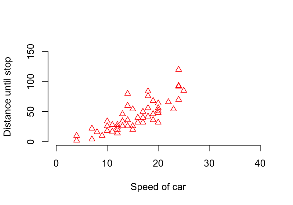
Figure 1.1: First plot of distance against speed in the cars dataset
In the above plot, we utilized R’s standard linear notation to tell it the relationship between variables. Thus, dist ~ speed can be interpreted statistically as dist is a function of speed. Note also the reference to the cars dataset in the call; without this call, we would need to write cars$dist ~ cars$speed. We can alter this plot in many ways, including the kinds of points, the labels, the axes, etc. Here is an example (figure 1.2).
plot(dist ~ speed, cars, pch = 2, col = "red", xlab = "Speed of car (mph)",
  ylab = "Distance until stop (ft)", xlim = c(0,40), ylim = c(0, 150), bty = "n")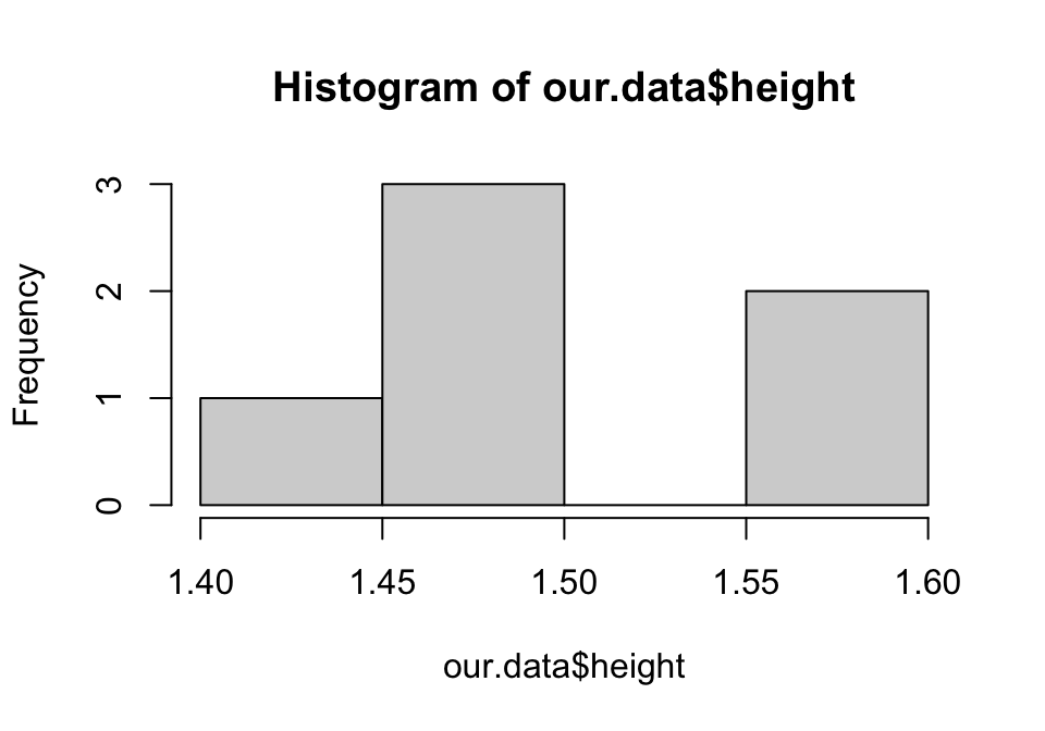
Figure 1.2: Second plot of distance against speed in the cars dataset
We can also try using the hist() function to create a histogram, for example to look at height by gender in our own dataset (figure 1.3).
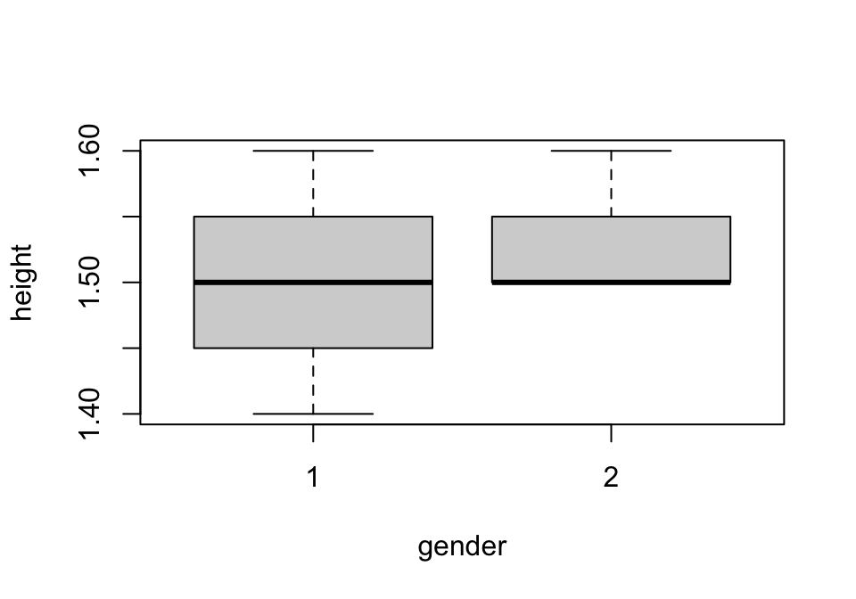
Figure 1.3: Histogram of sample height data
The hist() function can also be modified in a variety of important ways, using similar inputs to plot().
Let’s now see what the default plot style is for our gender-height data (figure 1.4).

Figure 1.4: Box-whisker plot of sample height data
We can see that the default here is a box-and-whisker plot, which is standard when we incorporate an x term that is categorical and a y term that is quantitative and continuous.
Now that we’ve explored a simple method of getting data into R, what about importing spreadsheets of demographic data? Although other methods certainly exist, we are particularly partial to the read.csv() function approach. This function allows us to import our data as a comma-separated value (CSV) text file. To utilize this approach, first open your preferred spreadsheet program and make sure that the data file meets the following conformational characteristics:
- The variables in your dataset are arranged by column, and the data points themselves are arranged by row.
- The top row in your spreadsheet contains ONLY the names of your variables, and these variable names conform to R object naming conventions (i.e. each variable name is unique, each variable name starts with a letter or underscore only, each variable name includes no punctuation other than the period).
- The data sheet itself does not contain ANY commas anywhere.
- All columns intended to be numeric variables contain ONLY numeric entries or blanks, except for the cell holding the variable name (even a single text entry in a single column will cause the column to be imported as a string variable).
- The dataset must start with the very top-left cell in the spreadsheet. Starting everything lower than the first row or further to the right than the first column will cause improper importing and formatting issues.
- The dataset does not include any characters other than pure ASCII characters. While R can handle UTF-8 and some other kinds of text encoding, some methods produce unexpected behavior when handling values or objects named with non-ASCII encoding.
Once your dataset conforms to these parameters in the spreadsheet program, export your file to CSV format (we generally encourage MS-DOS CSV format, if such an option is provided, as it is the simplest version). Then, in R, use the following command to import your dataset, replacing myfilenamehere with the real file name:
Once done, try using the summary() function to see what everything looks like and whether the variables were imported properly. You can also use the dim() function to see the numbers of rows and columns imported. Clicking on the resulting structure in the Environment pane will also open the data frame into the top-left RStudio panel to allow more thorough exploration.
Let’s now move on to using lefko3 itself.
1.7 Using lefko3
Users of lefko3 will first need to install the package itself. The following line of code will do that. The user should agree to install a number of other packages stated as dependencies, if prompted. The specific dependencies currently include BH, glmmTMB, lme4, Matrix, MuMIn, pscl, Rcpp, RcppArmadillo, stringr, TMB, and VGAM, and they should be installed similarly if not prompted and if not installed. Note that lefko3 is also meant to work with the newest version of R, and the newest versions of these dependencies. It has been tested with versions of R as far back as 3.5.0 and so should work with those, but it is possible that dependency upgrades will affect certain functions (most importantly modelsearch(), which is dependent on virtually all of the packages noted above).
Alternatively, development versions of lefko3 are available on r-universe (https://dormancy1.r-universe.dev/lefko3), where updates are more frequent than on CRAN. Development versions are not always stable, while CRAN versions are, but users wishing to try new features prior to a new stable release can install lefko3 with the following line.
install.packages('lefko3', repos = c('https://dormancy1.r-universe.dev', 'https://cloud.r-project.org'))
Once installed, use of lefko3 requires loading it into the working environment, which can be done with the following line.
Package lefko3 includes functions to handle the entire workflow of MPM construction and analysis. The functions themselves can be divided into at least 8 major categories, as below:
Data transformation and handling functions
add_lM(): Adds new matrices to existing MPMs.append_lP(): Appends projection structures derived from the same life history together.
bootstrap3(): Creates lists of data frames bootstrapped from the same source data frame.delete_lM(): Deletes matrices from MPMs.historicalize3(): Formats demographic datasets that are in vertical but not historical format into a standardized format for use by the package.subset_lM(): Creates MPMs from matrices in other MPMs.verticalize3(): Formats demographic datasets that are in horizontal format into a standardized format for use by the package..
Functions setting or determining population characteristics for analysis
density_input(): Summarizes density dependence inputs for population projection.density_vr(): Summarizes density dependence inputs in vital rates for function-based population projection.hfv_qc(): Tests assumptions of various response distributions in key vital rate variables in demographic datasets.sf_create(): Creates a data frame summarizing the life history model.sf_distrib(): Tests for overdispersion and zero-inflation in count-based size and fecundity.sf_skeleton(): Creates a stageframe skeleton.stage_weight(): Determines contribution of stages to population size for density dependence calculations.start_input(): Creates a start vector for population projection.summary_hfv(): Summarizes key information about properly formatted demographic datasets.supplemental(): Summarizes extra inputs for MPM creation not found within the demographic dataset.
Vital rate model building and selection
create_pm(): Creates a skeleton data frame indexing variables used in vital rate modeling.miniMod(): Takes modelsearch() output and translates it intovrm_inputobjects, which can potentially save vast amounts of memory.
modelsearch(): Creates best-fit vital rate models for function-based MPMs, and to test the influences of individual history and other factors.vrm_import(): Imports coefficients from linear vital rate models for use in developing discretized IPMs and function-based MPMs.
Matrix / integral projection model creation and import functions
aflefko2(): Constructs function-based ahistorical age-by-stage MPMs.arlefko2(): Constructs raw ahistorical age-by-stage MPMs.create_lM(): Creates MPMs from matrices provided by the user.flefko2(): Constructs ahistorical function-based MPMs.flefko3(): Constructs historical function-based MPMs.fleslie(): Constructs function-based Leslie MPMs.hist_null(): Constructs historically-formatted MPMs assuming no individual history.lmean(): Develops element-wise arithmetic mean MPMs.
mpm_create(): Constructs all forms of MPM.rlefko2(): Constructs ahistorical raw MPMs.rlefko3(): Constructs historical raw MPMs.rleslie(): Constructs raw Leslie MPMs.
Matrix / integral projection model editing functions
add_stage(): Adds new stages to existing MPMs.
edit_lM(): Edits matrices by element.
Population dynamics analysis functions
actualstage3(): Calculates observed population stage frequencies and proportions.elasticity3(): Estimates the deterministic or stochastic elasticities of population growth rate to matrix elements.f_projection3(): Core population projection function for time-by-time projection of function-based MPMs and IPMs from vital rate models.lambda3(): Estimates deterministic or stochastic population growth rate.ltre3(): Conducts deterministic, stochastic, and small noise approximation life table response experiments.projection3(): Core population projection function for already constructed MPMs and IPMs.repvalue3(): Estimates the deterministic stage reproductive values or stochastic long-run reproductive values.sensitivity3(): Estimates the deterministic or stochastic sensitivities of population growth rate to matrix elements.slambda3(): Estimates stochastic population growth rate.stablestage3(): Estimates the deterministic stable stage equilibrium or stochastic long-run stage distribution.
Functions describing, summarizing, comparing, or visualizing MPMs and derived structures.
cond_hmpm(): Extracts conditional ahistorical matrices from historical MPMs.cond_diff(): Develops conditional ahistorical difference matrices, given two sets of historical or historically-formatted MPMs as input.diff_lM(): Creates difference matrices between two MPMs with matrices of equal dimension.image3(): Creates images of MPMs, sensitivity matrices, elasticity matrices, and LTRE matrices.
Other useful functions.
beverton3(): The two-parameter Beverton-Holt function for scalars.logistic3(): The two-parameter logistic function for scalars.markov_run(): Develops vectors of shuffled times for use in setting matrix projections, assuming 1st order Markovian transitions among times.plot(): Displays plots of certain outputs, including population projections resulting from functionsprojection3()andf_projection3().ricker3(): The two-parameter Ricker function for scalars.summary(): Various versions of thesummary()function have been created to provide useful summaries of output from manylefko3functions.usher3(): The two-parameter Usher function for scalars.
In addition, lefko3 includes five datasets that can be used for educational purposes. These include anthyllis, cypdata, cypvert, lathyrus, and pyrola.
1.7.1 The lefkoMat object: organized MPMs and IPMs
Package lefko3 produces a number of different classes of S3 objects, which can be thought of as standardized lists used as input and output for its functions. The most fundamental of these is the lefkoMat object, which holds the MPM and associated metadata. This list object is made of the following elements.
A: A list of full population projection matrices, in order of population, patch, and year. Each matrix is either of classmatrixorMatrixclassdgCMatrix(the latter is sparse matrix format).U: A list of matrices showing only survival-transition elements, in the same order as A.F: A list of matrices showing only fecundity elements, in the same order as A.hstages: A data frame showing the order of paired stages (given if matrices are historical, otherwiseNA).agestages: A data frame showing the order of age-stages (if an age-by-stage MPM has been created, otherwiseNA).ahstages: A data frame detailing the characteristics of the life history model used for construction of the MPM.labels: A data frame showing the order of matrices, according to population, patch, and year.matrixqc: A vector used insummarystatements to describe the overall quality of each matrix.dataqc: A vector used insummarystatements to describe key sampling aspects of the dataset (in raw MPMs).modelqc: A vector used insummarystatements to describe the vital rate models (in function-based MPMs).
Objects within these lists may be called as in figure 1.5, below.
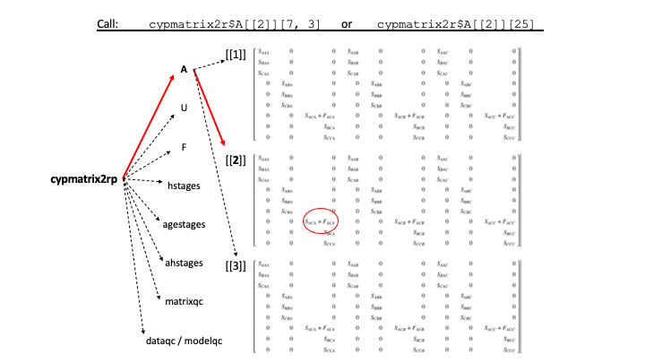
We will detail the creation and meaning of these objects in later chapters, but for now let’s construct a simple MPM as a lefkoMat object. For this purpose, we will input the first six matrices of the MPM analyzed in Davison et al. (2010). This example will focus on just two populations of Anthyllis vulneraria, an herbaceous plant studied in south-western Belgium. First we will create the stageframe, which summarizes the life history model of the plant (stageframes and life history models will be described in Chapter 2).
sizevector <- c(1, 1, 2, 3) # These sizes are not from the original paper
stagevector <- c("Sdl", "Veg", "SmFlo", "LFlo")
repvector <- c(0, 0, 1, 1)
obsvector <- c(1, 1, 1, 1)
matvector <- c(0, 1, 1, 1)
immvector <- c(1, 0, 0, 0)
propvector <- c(0, 0, 0, 0)
indataset <- c(1, 1, 1, 1)
binvec <- c(0.5, 0.5, 0.5, 0.5)
comments <- c("Seedling", "Vegetative adult", "Small flowering",
  "Large flowering")

anthframe <- sf_create(sizes = sizevector, stagenames = stagevector,
  repstatus = repvector, obsstatus = obsvector, matstatus = matvector,
  immstatus = immvector, indataset = indataset, binhalfwidth = binvec,
  propstatus = propvector, comments = comments)

class(anthframe)
> [1] "data.frame" "stageframe"
anthframe
>   stage size size_b size_c min_age max_age repstatus obsstatus propstatus
> 1   Sdl    1     NA     NA      NA      NA         0         1          0
> 2   Veg    1     NA     NA      NA      NA         0         1          0
> 3 SmFlo    2     NA     NA      NA      NA         1         1          0
> 4  LFlo    3     NA     NA      NA      NA         1         1          0
>   immstatus matstatus indataset binhalfwidth_raw sizebin_min sizebin_max
> 1         1         0         1              0.5         0.5         1.5
> 2         0         1         1              0.5         0.5         1.5
> 3         0         1         1              0.5         1.5         2.5
> 4         0         1         1              0.5         2.5         3.5
>   sizebin_center sizebin_width binhalfwidthb_raw sizebinb_min sizebinb_max
> 1              1             1                NA           NA           NA
> 2              1             1                NA           NA           NA
> 3              2             1                NA           NA           NA
> 4              3             1                NA           NA           NA
>   sizebinb_center sizebinb_width binhalfwidthc_raw sizebinc_min sizebinc_max
> 1              NA             NA                NA           NA           NA
> 2              NA             NA                NA           NA           NA
> 3              NA             NA                NA           NA           NA
> 4              NA             NA                NA           NA           NA
>   sizebinc_center sizebinc_width group         comments
> 1              NA             NA     0         Seedling
> 2              NA             NA     0 Vegetative adult
> 3              NA             NA     0  Small flowering
> 4              NA             NA     0  Large flowering
This object, called anthframe, is a data frame in R. Checking its class reveals that it is also a member of the class stageframe, which is a kind of data frame unique to lefko3 having the particular structure seen here. This object was created by developing a number of vectors describing the life history stages that this plant lives through, and using these as inputs into the stageframe creation function, sf_create().
Now let’s input three matrices each for two populations, both of which are part of a metapopulation. The three matrices show transitions across pairs of consecutive years, 2003-2004, 2004-2005, and 2005-2006. We input these matrices by row because the code supplied in Davison et al. (2010) was written in Matlab, which defaults to input by row.
# POPN C 2003-2004
XC3 <- matrix(c(0, 0, 1.74, 1.74,
  0.208333333, 0, 0, 0.057142857,
  0.041666667, 0.076923077, 0, 0,
  0.083333333, 0.076923077, 0.066666667, 0.028571429), 4, 4, byrow = TRUE)

# POPN C 2004-2005
XC4 <- matrix(c(0, 0, 0.3, 0.6,
0.32183908, 0.142857143, 0, 0,
0.16091954, 0.285714286, 0, 0,
0.252873563, 0.285714286, 0.5, 0.6), 4, 4, byrow = TRUE)

# POPN C 2005-2006
XC5 <- matrix(c(0, 0, 0.50625, 0.675,
0, 0, 0, 0.035714286,
0.1, 0.068965517, 0.0625, 0.107142857,
0.3, 0.137931034, 0, 0.071428571), 4, 4, byrow = TRUE)

# POPN E 2003-2004
XE3 <- matrix(c(0, 0, 2.44, 6.569230769,
0.196428571, 0, 0, 0,
0.125, 0.5, 0, 0,
0.160714286, 0.5, 0.133333333, 0.076923077), 4, 4, byrow = TRUE)

# POPN E 2004-2005
XE4 <- matrix(c(0, 0, 0.45, 0.646153846,
0.06557377, 0.090909091, 0.125, 0,
0.032786885, 0, 0.125, 0.076923077,
0.049180328, 0, 0.125, 0.230769231), 4, 4, byrow = TRUE)

# POPN E 2005-2006
XE5 <- matrix(c(0, 0, 2.85, 3.99,
0.083333333, 0, 0, 0,
0, 0, 0, 0,
0.416666667, 0.1, 0, 0.1), 4, 4, byrow = TRUE)
Let’s take a quick look at one of these matrices.
XC3
>            [,1]       [,2]       [,3]       [,4]
> [1,] 0.00000000 0.00000000 1.74000000 1.74000000
> [2,] 0.20833333 0.00000000 0.00000000 0.05714286
> [3,] 0.04166667 0.07692308 0.00000000 0.00000000
> [4,] 0.08333333 0.07692308 0.06666667 0.02857143
Note that the structure is very conventional - the fecundity rates are in the top-right corner, while the rest of the matrix shows transition probabilities with elements bound between 0 and 1. All MPM matrices should contain only non-negative values, so we recommend inspecting your matrices when you construct them.
Next, we will make a list of our matrices, and then use the create_lM() function to create our lefkoMat object. We will also supply vectors showing the order of patches in the list of matrices, and the order of year at time t in the list of matrices (ahistorical matrices show transition rates from time t to time t+1, so the matrix covering 2004-2005 is referred to by year 2004). Because lefko3 includes special methods to build and analyze historical MPMs, we will tell R that these matrices are not historical (historical = FALSE).
mats_list <- list(XC3, XC4, XC5, XE3, XE4, XE5)

anth_lefkoMat <- create_lM(mats_list, anthframe, historical = FALSE,
  patchorder = c(1, 1, 1, 2, 2, 2),
  yearorder = c(2003, 2004, 2005, 2003, 2004, 2005))
> Warning: No supplement provided. Assuming fecundity yields all propagule and
> immature stages.

anth_lefkoMat
> $A
> $A[[1]]
>            [,1]       [,2]       [,3]       [,4]
> [1,] 0.00000000 0.00000000 1.74000000 1.74000000
> [2,] 0.20833333 0.00000000 0.00000000 0.05714286
> [3,] 0.04166667 0.07692308 0.00000000 0.00000000
> [4,] 0.08333333 0.07692308 0.06666667 0.02857143
>
> $A[[2]]
>           [,1]      [,2] [,3] [,4]
> [1,] 0.0000000 0.0000000  0.3  0.6
> [2,] 0.3218391 0.1428571  0.0  0.0
> [3,] 0.1609195 0.2857143  0.0  0.0
> [4,] 0.2528736 0.2857143  0.5  0.6
>
> $A[[3]]
>      [,1]       [,2]    [,3]       [,4]
> [1,]  0.0 0.00000000 0.50625 0.67500000
> [2,]  0.0 0.00000000 0.00000 0.03571429
> [3,]  0.1 0.06896552 0.06250 0.10714286
> [4,]  0.3 0.13793103 0.00000 0.07142857
>
> $A[[4]]
>           [,1] [,2]      [,3]       [,4]
> [1,] 0.0000000  0.0 2.4400000 6.56923077
> [2,] 0.1964286  0.0 0.0000000 0.00000000
> [3,] 0.1250000  0.5 0.0000000 0.00000000
> [4,] 0.1607143  0.5 0.1333333 0.07692308
>
> $A[[5]]
>            [,1]       [,2]  [,3]       [,4]
> [1,] 0.00000000 0.00000000 0.450 0.64615385
> [2,] 0.06557377 0.09090909 0.125 0.00000000
> [3,] 0.03278689 0.00000000 0.125 0.07692308
> [4,] 0.04918033 0.00000000 0.125 0.23076923
>
> $A[[6]]
>            [,1] [,2] [,3] [,4]
> [1,] 0.00000000  0.0 2.85 3.99
> [2,] 0.08333333  0.0 0.00 0.00
> [3,] 0.00000000  0.0 0.00 0.00
> [4,] 0.41666667  0.1 0.00 0.10
>
>
> $U
> $U[[1]]
>            [,1]       [,2]       [,3]       [,4]
> [1,] 0.00000000 0.00000000 0.00000000 0.00000000
> [2,] 0.20833333 0.00000000 0.00000000 0.05714286
> [3,] 0.04166667 0.07692308 0.00000000 0.00000000
> [4,] 0.08333333 0.07692308 0.06666667 0.02857143
>
> $U[[2]]
>           [,1]      [,2] [,3] [,4]
> [1,] 0.0000000 0.0000000  0.0  0.0
> [2,] 0.3218391 0.1428571  0.0  0.0
> [3,] 0.1609195 0.2857143  0.0  0.0
> [4,] 0.2528736 0.2857143  0.5  0.6
>
> $U[[3]]
>      [,1]       [,2]   [,3]       [,4]
> [1,]  0.0 0.00000000 0.0000 0.00000000
> [2,]  0.0 0.00000000 0.0000 0.03571429
> [3,]  0.1 0.06896552 0.0625 0.10714286
> [4,]  0.3 0.13793103 0.0000 0.07142857
>
> $U[[4]]
>           [,1] [,2]      [,3]       [,4]
> [1,] 0.0000000  0.0 0.0000000 0.00000000
> [2,] 0.1964286  0.0 0.0000000 0.00000000
> [3,] 0.1250000  0.5 0.0000000 0.00000000
> [4,] 0.1607143  0.5 0.1333333 0.07692308
>
> $U[[5]]
>            [,1]       [,2]  [,3]       [,4]
> [1,] 0.00000000 0.00000000 0.000 0.00000000
> [2,] 0.06557377 0.09090909 0.125 0.00000000
> [3,] 0.03278689 0.00000000 0.125 0.07692308
> [4,] 0.04918033 0.00000000 0.125 0.23076923
>
> $U[[6]]
>            [,1] [,2] [,3] [,4]
> [1,] 0.00000000  0.0    0  0.0
> [2,] 0.08333333  0.0    0  0.0
> [3,] 0.00000000  0.0    0  0.0
> [4,] 0.41666667  0.1    0  0.1
>
>
> $F
> $F[[1]]
>      [,1] [,2] [,3] [,4]
> [1,]    0    0 1.74 1.74
> [2,]    0    0 0.00 0.00
> [3,]    0    0 0.00 0.00
> [4,]    0    0 0.00 0.00
>
> $F[[2]]
>      [,1] [,2] [,3] [,4]
> [1,]    0    0  0.3  0.6
> [2,]    0    0  0.0  0.0
> [3,]    0    0  0.0  0.0
> [4,]    0    0  0.0  0.0
>
> $F[[3]]
>      [,1] [,2]    [,3]  [,4]
> [1,]    0    0 0.50625 0.675
> [2,]    0    0 0.00000 0.000
> [3,]    0    0 0.00000 0.000
> [4,]    0    0 0.00000 0.000
>
> $F[[4]]
>      [,1] [,2] [,3]     [,4]
> [1,]    0    0 2.44 6.569231
> [2,]    0    0 0.00 0.000000
> [3,]    0    0 0.00 0.000000
> [4,]    0    0 0.00 0.000000
>
> $F[[5]]
>      [,1] [,2] [,3]      [,4]
> [1,]    0    0 0.45 0.6461538
> [2,]    0    0 0.00 0.0000000
> [3,]    0    0 0.00 0.0000000
> [4,]    0    0 0.00 0.0000000
>
> $F[[6]]
>      [,1] [,2] [,3] [,4]
> [1,]    0    0 2.85 3.99
> [2,]    0    0 0.00 0.00
> [3,]    0    0 0.00 0.00
> [4,]    0    0 0.00 0.00
>
>
> $hstages
> [1] NA
>
> $agestages
> [1] NA
>
> $ahstages
>   stage_id stage_id stage original_size original_size_b original_size_c min_age
> 1        1        1   Sdl             1              NA              NA       0
> 2        2        2   Veg             1              NA              NA       0
> 3        3        3 SmFlo             2              NA              NA       0
> 4        4        4  LFlo             3              NA              NA       0
>   max_age repstatus obsstatus propstatus immstatus matstatus entrystage
> 1      NA         0         1          0         1         0          1
> 2      NA         0         1          0         0         1          0
> 3      NA         1         1          0         0         1          0
> 4      NA         1         1          0         0         1          0
>   indataset binhalfwidth_raw sizebin_min sizebin_max sizebin_center
> 1         1              0.5         0.5         1.5              1
> 2         1              0.5         0.5         1.5              1
> 3         1              0.5         1.5         2.5              2
> 4         1              0.5         2.5         3.5              3
>   sizebin_width binhalfwidthb_raw sizebinb_min sizebinb_max sizebinb_center
> 1             1                NA           NA           NA              NA
> 2             1                NA           NA           NA              NA
> 3             1                NA           NA           NA              NA
> 4             1                NA           NA           NA              NA
>   sizebinb_width binhalfwidthc_raw sizebinc_min sizebinc_max sizebinc_center
> 1             NA                NA           NA           NA              NA
> 2             NA                NA           NA           NA              NA
> 3             NA                NA           NA           NA              NA
> 4             NA                NA           NA           NA              NA
>   sizebinc_width group         comments alive almostborn
> 1             NA     0         Seedling     1          0
> 2             NA     0 Vegetative adult     1          0
> 3             NA     0  Small flowering     1          0
> 4             NA     0  Large flowering     1          0
>
> $labels
>   pop patch year2
> 1   1     1  2003
> 2   1     1  2004
> 3   1     1  2005
> 4   1     2  2003
> 5   1     2  2004
> 6   1     2  2005
>
> $matrixqc
> [1] 44 12  6
>
> $dataqc
> [1] NA NA
>
> attr(,"class")
> [1] "lefkoMat"
Voilà! We are now free to use this MPM in our analyses. But before we do that we might wish to explore this structure a bit more. The first element of this lefkoMat object, named A, is a list of the actual projection matrices. The create_lM() function uses the stageframe input that we provided to ascertain which transition rates are survival probabilities and which correspond to fecundity rates. The element named U is a list including a survival-transition matrix for each A matrix, meaning that fecundity is removed. The F element is a list including a fecundity matrix for each A matrix, meaning that survival transition probabilities have been removed. The element ahstages is our stageframe, though slightly edited and reordered. Here, element hstages is just NA, but would include the order of historical stage pairs if this MPM was historical. Element agestages is also NA, but would show us the order of age-stage combinations if this were an age-by-stage MPM or a Leslie MPM. The final element, matrixqc includes some basic quality control data in vector format. All of this is summarized using the summary() function, as below.
summary(anth_lefkoMat)
>
> This ahistorical lefkoMat object contains 6 matrices.
>
> Each matrix is square with 4 rows and columns, and a total of 16 elements.
> A total of 44 survival transitions were estimated, with 7.333 per matrix.
> A total of 12 fecundity transitions were estimated, with 2 per matrix.
> This lefkoMat object covers 1 population, 2 patches, and 3 time steps.
>
> This lefkoMat object appears to have been imported. Number of unique individuals and transitions not known.
>
> Survival probability sum check (each matrix represented by column in order):
>           [,1]  [,2]   [,3]   [,4]   [,5]  [,6]
> Min.    0.0667 0.500 0.0625 0.0769 0.0909 0.000
> 1st Qu. 0.0810 0.575 0.1708 0.1192 0.1334 0.075
> Median  0.1198 0.657 0.2106 0.3077 0.2276 0.100
> Mean    0.1599 0.637 0.2209 0.4231 0.2303 0.175
> 3rd Qu. 0.1987 0.720 0.2607 0.6116 0.3245 0.200
> Max.    0.3333 0.736 0.4000 1.0000 0.3750 0.500
>
>
> Stages without connections leading to the rest of the life cycle found in matrices: 5
Summaries such as this are quite useful. Here we can see how many matrices we have (corresponding to A matrices), how big each matrix is, how many elements were estimated on average per matrix and across the board (the numbers of estimated elements shown actually shows us the number of non-zero elements, and so it is possible that the number of estimated elements is actually larger if some elements were estimated as 0), and how many populations, patches / subpopulations, and time steps are covered. This is followed by a summary of the column sums of the corresponding U matrices - this is an important quality control check because all numbers within the U matrices should conform to \(0 \le a_{ij} \le 1\), where \(a_{ij}\) is the element at row \(i\) and column \(j\), and all column sums within these matrices should also conform to \(0 \le \sum_i a_{ij} \le 1\), where \(\sum_i a_{ij}\) is the sum of all elements in column \(j\) and corresponds to the survival probability of stage \(j\).
1.8 Datasets used in this book
This book will utilize five main datasets. The first and second datasets are data frames holding individual-level monitoring data on a population of the North American orchid species Cypripedium candidum, also known as the white lady’s slipper. Both are the same dataset, but formatted differently. The third dataset is a data frame holding similar data for a population of the European perennial Lathyrus vernus. The fourth dataset is a lefkoMat object holding projection matrices from nine populations of from the European perennial Anthyllis vulneraria. The fifth and final dataset is a data frame holding demographic data on a population each of Pyrola japonica and Pyrola subaphylla from Fukushima Prefecture, Japan.
1.8.1 Cypripedium candidum data
This dataset is available in two formats, as data frames called cypdata and cypvert. These datasets contain the exact same information and are in different formats only. They can be called with the following code.
The white lady’s slipper, Cypripedium candidum, is a North American perennial herb in the family Orchidaceae. It is long-lived and of conservation concern. This plant begins life by germinating from a dust seed, and then develops into a protocorm, which is a special subterranean life stage found in orchids and pyroloids. During this stage, the plant is non-photosynthetic and completely parasitic on its mycorrhizal fungi. It spends several years as a protocorm, and previous studies suggest that it typically spends 3 years before becoming a seedling. As a seedling, it may or may not produce aboveground sprouts, often remaining entirely subterranean and continuing its parasitic lifestyle. It may persist this way for many years before attaining adult size, at which point it may sprout with or without flowers, or may remain underground in a condition referred to as vegetative dormancy. The latter condition may continue for many years, with over a decade of continuous dormancy documented in the literature (Shefferson et al. 2018).
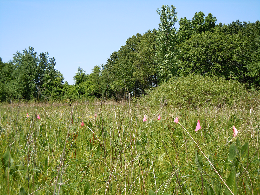
lefko3. Photo courtesy of R. SheffersonThe population from which the dataset originates is located within a wet meadow in a state nature preserve located in northeastern Illinois, USA (Figure 1.6). The population was monitored annually from 2004 to 2009, with two monitoring sessions per year. Monitoring sessions took roughly 2 weeks each, and included complete censuses of the population divided into sections referred to as patches. Each monitoring session consisted of searches for previously recorded individuals, which were located according to coordinates relative to fixed stakes at the site, followed by a search for new individuals. Data recorded per individual included: the location, the number of non-flowering sprouts, the number of flowering sprouts, the number of flowers per flowering sprout, and the number of fruit pods per sprout (only in the second monitoring session per year, once fruiting had occurred). Location was used to infer individual identity. More information about this population and its characteristics is given in Shefferson et al. (2001) and Shefferson et al. (2017).
1.8.2 Lathyrus vernus data
This dataset is available as a data frame called lathyrus, and can be called with the following code.
Lathyrus vernus (family Fabaceae) is a long-lived forest herb, native to Europe and large parts of northern Asia. Individuals increase slowly in size and usually flower only after 10-15 years of vegetative growth. Flowering individuals have an average conditional lifespan of 44.3 years (Ehrlén & Lehtila 2002). L. vernus lacks organs for vegetative spread and individuals are well delimited (Ehrlén 2002). One or several erect shoots of up to 40 cm height emerge from a subterranean rhizome in March-April. Flowering occurs about four weeks after shoot emergence. Shoot growth is determinate, and the number of flowers is determined in the previous year (Ehrlén & Van Groenendael 2001). Individuals may not produce aboveground structures every year, but can remain dormant in one or more seasons. L. vernus is self-compatible but requires visits from bumble-bees to produce seeds. Individuals produce few, large seeds and establishment from seeds is relatively frequent (Ehrlén & Eriksson 1996). The pre-dispersal seed predator Bruchus atomarius often consumes a large fraction of developing seeds, and roe deer (Capreolus capreolus) sometimes consume the shoots (Ehrlén & Munzbergova 2009).
Data for this study were collected from six permanent plots in a population of L. vernus located in a deciduous forest in the Tullgarn area, SE Sweden (58.9496 N, 17.6097 E), during 1988–1991 (Ehrlén 1995). The six plots were similar with regard to soil type, elevation, slope, and canopy cover. Within each plot, all individuals were marked with numbered tags that remained over the study period, and their locations were carefully mapped. New individuals were included in the study in each year. Individuals were recorded at least three times every growth season. At the time of shoot emergence, we recorded whether individuals were alive and produced above-ground shoots, and if shoots had been grazed. During flowering, we recorded flower number and the height and diameter of all shoots. At fruit maturation, we counted the number of intact and damaged seeds. To derive a measure of above-ground size for each individual, we calculated the volume of each shoot as \(\pi × (\frac{1}{2} diameter)^2 × height\), and summed the volumes of all shoots. This measure is closely correlated with the dry mass of aboveground tissues (\(R^2 = 0.924\), \(P < 0.001\), \(n = 50\), log-transformed values; Ehrlén 1995). Size of individuals that had been grazed was estimated based on measures of shoot diameter in grazed shoots, and the relationship between shoot diameter and shoot height in non-grazed individuals. Only individuals with an aboveground volume of more than 230 mm3 flowered and produced fruits during this study. Individuals that lacked aboveground structures in one season but reappeared in the following year were considered dormant. Individuals that lacked aboveground structures in two subsequent seasons were considered dead from the year in which they first lacked aboveground structures. Probabilities of seeds surviving to the next year, and of being present as seedlings or seeds in the soil seed bank, were derived from separate yearly sowing experiments in separate plots adjacent to each subplot (Ehrlén & Eriksson 1996).
1.8.3 Anthyllis vulneraria data
Davison et al. (2010) reported stochastic contributions made by differences in vital rate means and variances among nine natural populations of Anthyllis vulneraria, also known as kidney vetch. This plant occurs in calcareous grasslands in the Viroin Valley of south-western Belgium. A. vulneraria is a grassland specialist and the unique host plant of the Red-listed blue butterfly (Cupido minimus). It is a short-lived, rosette-forming legume with a complex life cycle but no seedbank.
Nine populations (N = 27-50,000) growing in distinct grassland fragments were surveyed between 2003 and 2006, yielding three (4x4) annual transition matrices for each population. The populations occurred within grassland fragments, and were mostly managed as nature reserves through rotational sheep grazing. These surveys coincided with a summer heat wave (2003), followed by a spring drought (2005) and an even more extreme heat wave (2006). These populations have been subject to detailed study for aspects of their genetics and demography, and further details on the sites can be obtained through the resulting publications (Krauss et al. 2004; Honnay et al. 2006; Piessens et al. 2009). We use the matrices published in Davison et al. (2010) to illustrate some of the features of lefko3, and so provide these matrices in a lefkoMat object (section 1.7.1).
1.8.4 Pyrola data
Shefferson et al. (2024) reported on two species of Pyrola, P. japonica and P. subaphylla, growing in western Fukushima Prefecture, Japan. These perennial herb species are partially mycoheterotrophic, with P. subaphylla exhibiting carbon and nitrogen isotope ratios suggesting near full mycoheterotrophy, while P. japonica exhibits isotopes suggesting a greater use of photosynthesis. Current taxonomy treats these two species as sisters, making them interesting for comparison to understand the evolution of mycoheterotrophy.
This demographic field study began in the summer / autumn of 2015 at two field sites roughly 20-25km apart. One site was home to the P. jaonica population, and the other was home to the P. subaphylla population. Both communities were mixed confierous / deciduous forests with sparse, rocky ground cover. The study continued through the autumn of 2020, for a total of six years of demographic data. Field work took roughly a week each year, and involved finding and measuring the numbers and sizes of leaves, inflorescences, and flowers and fruits. The plants are typically small, and are capable of vegetative dormancy. They germinate from dust seeds, and typically spend the first few years as subterranean seedlings.
1.9 Points to remember
- R is an object-oriented language using the atomic vector as its basic unit of analysis.
- RStudio provides an easy-to-use, convenient working environment for R analyses, including analyses using
lefko3. - Package
lefko3provides R with convenient, standardized objects organizing all aspects of the MPM creation and analysis process. It also provides powerful functions that develop and analyze MPMs using lightning fast binaries. - Package
lefko3incorporates five key datasets for use in all examples, vignettes, and the chapters of this book. - Package
lefko3does not currently work with tidyverse structures. Please use base R and Matrix structures when using this package.